Quantcast
Channel: rOpenSci - open tools for open science
Viewing all 668 articles
Browse latest View live

Release 'open' data from their PDF prisons using tabulizer

$
0
0

There is no problem in science quite as frustrating as other peoples' data. Whether it's malformed spreadsheets, disorganized documents, proprietary file formats, data without metadata, or any other data scenario created by someone else, scientists have taken to Twitter to complain about it. As a political scientist who regularly encounters so-called "open data" in PDFs, this problem is particularly irritating. PDFs may have "portable" in their name, making them display consistently on various platforms, but that portability means any information contained in a PDF is irritatingly difficult to extract computationally. Encountering "open data" PDFs therefore makes me shout things like this repeatedly:

What can we do about such data other than extract it by hand? One answer is rely on tabulizer a package I submitted to rOpenSci that reduces some and often all of the hassle of extracting tabular data locked inside PDFs.

What is tabulizer?

tabulizer provides R bindings to the tabula-java library, the open-source java library that powers Tabula (source code on GitHub). What this means is that tabulizer relies directly on the underlying java classes that power Tabula without the need for system calls or the need to explicitly install Tabula on your system. (A potential downside is the need to handle intricacies of rJava - R's interface to Java, which I discuss in depth below.)

Tabula is an extremely powerful tool for extracting tabular data locked in PDFs. It's an incredibly valuable tool because the PDF file specification does not have a "table" representation. Instead, PDFs simply represent tables through the fixed positioning of text into rows and columns. Thus, unlike HTML, Word (.docx), or Open Document (.odt) file formats, there is no easy programmatic way to identify a table in a PDF. Tabula thus implements novel algorithms for identifying rows and columns of data and extracting them. tabulizer just provides a thin R layer on top of this power Java code.

Unfortunately, this means that tabulizer is not a universal solution to data trapped in PDFs. In particular, it can only identify and extract tables that are represented as text in a PDF:

If a PDF is a scan of a document or the table is actually an image embedded in the PDF, tabula - and thus tabulizer - are useless. In those cases, users might want to check out the OCR functionality of tesseract, which Jeroen Ooms developed for rOpenSci and discussed previously on this blog.

But it does mean that a substantial amount of difficult-to-parse tabular information in PDFs is now readily and quickly accessible via just one tabulizer function: extract_tables().

Installation

tabulizer is not yet on CRAN. (It's CRAN-ready but due to some underlying developments that are ongoing in the tabula-java library, I'm waiting for a formal release.) In the meantime, it's possible to install tabulizer directly from GitHub.

Before doing that, I would encourage users to make sure they have rJava installed (from CRAN) and that it works correctly on their platform. A lot of users report difficulties installing tabulizer that ultimately boil down to being Java and rJava issues that need to be resolved first. The package README provides a number of details on installation, which requires a strictly ordered set of steps:

  1. Install the Java Development Kit, if you don't already have it on your system. (Note that the JDK is different from the Java Runtime Environment (JRE) that you almost certainly already have.) Details of how to do this vary a lot between platforms, so see the README for details.
  2. Install rJava using install.packages("rJava") and resolve any issues surrounding the JAVA_HOME environment variable that may need to be set before and/or after installing rJava. Again, see the README or various question/answer pairs on StackOverflow for platform-specific instructions.
  3. Install tabulizer and tabulizerjars (the package containing the tabula java library) using your favorite GitHub package installer:
library("ghit")
ghit::install_github(c("ropensci/tabulizerjars","ropensci/tabulizer"))

This should work. If not, set verbose = TRUE in ghit::install_github() to identify the source of any issues. Some common problems are the dependency on the png package, which might need to be installed first. On Windows (depending on your version of R and how it was installed) may require setting INSTALL_opts = "--no-multiarch" in ghit::install_github().

If none of these steps work, scroll through the GitHub issues page for anyone experiencing a similar problem and, if not resolved in any of those discussions, feel free to open an issue on GitHub describing your problem including the fully verbose output of install_github() and your sessionInfo().

Unlocking elections data with tabulizer

Elections data are the bread and butter of a lot of quantitative political science research. Many researchers in my field need to know how many citizens voted and for whom in order to make sense of campaigns, election integrity, partisanship, and so forth. Yet a substantial amount of election-related data is locked in government-produced PDFs. Worse, national, state, and local governments have little to no standardization in the formatting of elections data, meaning even if one could figure out a computational strategy for extracting one kind of data about elections in one year from one state, that computational strategy would likely be useless in the same state in another year or in any other state. Elections provide a fantastic and highly visible example of "open" government data that's not really open or usable at all.

As a simple example, this PDF from the California Secretary of State's office contains historical voter registration and turnout data in a well-formatted table. Why this is a PDF nobody knows. But extracting the tables using tabulizer's extract_tables() function is a breeze with no need to even download the file:

library("tabulizer")
sos_url <-"http://elections.cdn.sos.ca.gov/sov/2016-general/sov/04-historical-voter-reg-participation.pdf"
tab1 <- extract_tables(sos_url)
str(tab1)
## List of 2
##  $ : chr [1:58, 1:9] "" "Election Date" "Nov. 8, 1910" "Nov. 5, 1912 P" ...
##  $ : chr [1:6, 1:9] "" "Election Date" "Nov. 2, 2010" "Nov. 6, 2012 P" ...

The (default) result is a list of two matrices, each containing the tables from pages 1 and 2 of the document, respectively. A couple of quick cleanups and this becomes a well-formatted data frame:

# save header
h <- tab1[[1]][2,]# remove headers in first table
tab1[[1]]<- tab1[[1]][-c(1,2),]# remove duplicated header in second table
tab1[[2]]<- tab1[[2]][-c(1,2),]# merge into one table
tab1df <- setNames(as.data.frame(do.call("rbind", tab1), stringsAsFactors =FALSE), h)
str(tab1df)
## 'data.frame':    60 obs. of  9 variables:
##  $ Election Date: chr  "Nov. 8, 1910" "Nov. 5, 1912 P" "Nov. 3, 1914" "Nov. 7, 1916 P" ...
##  $ Eligible     : chr  "725,000" "1,569,000" "1,726,000" "1,806,000" ...
##  $ Democratic   : chr  "*" "*" "*" "*" ...
##  $ Republican   : chr  "*" "*" "*" "*" ...
##  $ Other        : chr  "*" "*" "*" "*" ...
##  $ Total        : chr  "*" "987,368" "1,219,345" "1,314,446" ...
##  $ Total Votes  : chr  "393,893" "707,776" "961,868" "1,045,858" ...
##  $ Registered   : chr  "*" "71.68%" "78.88%" "79.57%" ...
##  $ Eligible     : chr  "54.33%" "45.11%" "55.73%" "57.91%" ...

Which is very easy to then quickly turn into a time-series visualization of registration rates:

library("ggplot2")
years <-regexpr("[[:digit:]]{4}",tab1df[["Election Date"]])
tab1df$Year <-as.numeric(regmatches(tab1df[["Election Date"]], years))
tab1df$RegPerc <-as.numeric(gsub("%","", tab1df$Registered))
## Warning: NAs introduced by coercion
ggplot(tab1df, aes(x = Year, y = RegPerc))+
  geom_line()+ ylim(c(0,100))+ ylab("% Registered")+
  ggtitle("California Voter Registration, by Year")
## Warning: Removed 1 rows containing missing values (geom_path).

plot of chunk example1plot

Optional arguments

The extract_tables() has several arguments that control extraction and the return value of the function. They performed reasonably well here, but it's worth seeing a few of the other options. The method argument controls the return value. For extremely well-formatted tables, setting this to "data.frame" can be convenient, though it doesn't work perfectly here:

str(tab2 <- extract_tables(sos_url, method ="data.frame"))
## List of 2
##  $ :'data.frame':    57 obs. of  9 variables:
##   ..$ X        : chr [1:57] "Election Date" "Nov. 8, 1910" "Nov. 5, 1912 P" "Nov. 3, 1914" ...
##   ..$ X.1      : chr [1:57] "Eligible" "725,000" "1,569,000" "1,726,000" ...
##   ..$ X.2      : chr [1:57] "Democratic" "*" "*" "*" ...
##   ..$ X.3      : chr [1:57] "Republican" "*" "*" "*" ...
##   ..$ X.4      : chr [1:57] "Other" "*" "*" "*" ...
##   ..$ X.5      : chr [1:57] "Total" "*" "987,368" "1,219,345" ...
##   ..$ X.6      : chr [1:57] "Total Votes" "393,893" "707,776" "961,868" ...
##   ..$ Turnout  : chr [1:57] "Registered" "*" "71.68%" "78.88%" ...
##   ..$ Turnout.1: chr [1:57] "Eligible" "54.33%" "45.11%" "55.73%" ...
##  $ :'data.frame':    5 obs. of  9 variables:
##   ..$ X        : chr [1:5] "Election Date" "Nov. 2, 2010" "Nov. 6, 2012 P" "Nov. 4, 2014" ...
##   ..$ X.1      : chr [1:5] "Eligible" "23,551,699" "23,802,577" "24,288,145" ...
##   ..$ X.2      : chr [1:5] "Democratic" "7,620,240" "7,966,422" "7,708,683" ...
##   ..$ X.3      : chr [1:5] "Republican" "5,361,875" "5,356,608" "5,005,422" ...
##   ..$ X.4      : chr [1:5] "Other" "4,303,768" "4,922,940" "5,089,718" ...
##   ..$ X.5      : chr [1:5] "Total" "17,285,883" "18,245,970" "17,803,823" ...
##   ..$ X.6      : chr [1:5] "Total Votes" "10,300,392" "13,202,158" "7,513,972" ...
##   ..$ Turnout  : chr [1:5] "Registered" "59.59%" "72.36%" "42.20%" ...
##   ..$ Turnout.1: chr [1:5] "Eligible" "43.74%" "55.47%" "30.94%" ...

Setting method = "character" returns a list of character vectors with white space reflecting the positioning of text within the PDF's tabular representation:

str(tab3 <- extract_tables(sos_url, method ="character"))
## List of 2
##  $ : chr "\t\t\t\t\t\t\tTurnout\tTurnout\nElection Date\tEligible\tDemocratic\tRepublican\tOther\tTotal\tTotal Votes\tRegistered\tEligibl"| __truncated__

This argument can also be set to "csv", "tsv", or "json" to use a java-level utility to write the table to files in the working directory but this tends to be inconvenient. (For advanced users, method = "asis" returns an rJava object reference for those who want to manipulate the Java representation of the table directly.)

The other most important option to be aware of is guess, which indicates whether a column-finding algorithm should be used to identify column breaks. This should almost always be TRUE, setting it to FALSE will tend to return a less useful structure:

head(extract_tables(sos_url, guess =FALSE)[[1]],10)
##       [,1]
##  [1,] ""
##  [2,] ""
##  [3,] ""
##  [4,] ""
##  [5,] "Election Date"
##  [6,] "Nov. 8, 1910"
##  [7,] "Nov. 5, 1912 P"
##  [8,] "Nov. 3, 1914"
##  [9,] "Nov. 7, 1916 P"
## [10,] "Nov. 5, 1918"
##       [,2]
##  [1,] "HISTORICAL VOTER REGISTRATION AND"
##  [2,] "PARTICIPATION IN STATEWIDE GENERAL ELECTIONS 1910-2016"
##  [3,] "Registration Votes Cast"
##  [4,] "Turnout"
##  [5,] "Eligible Democratic Republican Other Total Total Votes Registered"
##  [6,] "725,000 * * * *393,893*"
##  [7,] "1,569,000 * * * 987,368 707,776 71.68%"
##  [8,] "1,726,000 * * * 1,219,345 961,868 78.88%"
##  [9,] "1,806,000 * * * 1,314,446 1,045,858 79.57%"
## [10,] "1,918,000 * * * 1,203,898 714,525 59.35%"
##       [,3]
##  [1,] ""
##  [2,] ""
##  [3,] ""
##  [4,] "Turnout"
##  [5,] "Eligible"
##  [6,] "54.33%"
##  [7,] "45.11%"
##  [8,] "55.73%"
##  [9,] "57.91%"
## [10,] "37.25%"

However, it can be useful if users want to specify the locations of tables manually. The area argument allows users to specifying a c(top,left,bottom,right) vector of coordinates for the location of tables on a page (which is useful if pages also contain other non-tabular content); setting columns with guess = FALSE indicates where the column breaks are within a table. With a little care in specifying column positions we can successfully separate the "P" flags specifying Presidential elections that were earlier concatenated with the election dates:

cols <-list(c(76,123,126,203,249,297,342,392,453,498,548))
tab4 <- extract_tables(sos_url, guess =FALSE, columns = cols)# save header
h <- tab4[[1]][5,-1]# clean tables
tab4[[1]]<- tab4[[1]][-c(1:5,62),-1]
tab4[[2]]<- tab4[[2]][-c(1:5,10:17),-1]# merge into one table
tab4df <- setNames(as.data.frame(do.call("rbind", tab4), stringsAsFactors =FALSE), h)
str(tab4df)
## 'data.frame':    60 obs. of  10 variables:
##  $ Election Date: chr  "Nov. 8, 1910" "Nov. 5, 1912" "Nov. 3, 1914" "Nov. 7, 1916" ...
##  $              : chr  "" "P" "" "P" ...
##  $ Eligible     : chr  "725,000" "1,569,000" "1,726,000" "1,806,000" ...
##  $ Democratic   : chr  "*" "*" "*" "*" ...
##  $ Republican   : chr  "*" "*" "*" "*" ...
##  $ Other        : chr  "*" "*" "*" "*" ...
##  $ Total        : chr  "*" "987,368" "1,219,345" "1,314,446" ...
##  $ Total Votes  : chr  "393,893" "707,776" "961,868" "1,045,858" ...
##  $ Registered   : chr  "*" "71.68%" "78.88%" "79.57%" ...
##  $ Eligible     : chr  "54.33%" "45.11%" "55.73%" "57.91%" ...

Figuring out columns positions and/or table areas is quite challenging to do by hand, so the locate_areas() provides an interactive interface for identifying areas. It returns lists of coordinates for specific table areas. A higher-level function, extract_areas(), connects that GUI directly to extract_tables() to return the tables within specified areas. Two other functions can be useful in this respect: get_n_pages() indicates the number of pages in a PDF and get_page_dims() indicates the dimensions of the pages.

Some other functionality

In addition to the core functionality around extract_tables(), tabulizer also provides some functions for working with PDFs that might be useful to those trapped in other peoples' data. We'll download the file first just to save some time:

tmp <-tempfile(fileext =".pdf")
download.file(sos_url, destfile = tmp, mode ="wb", quiet =TRUE)

The extract_text() function extracts text content of the PDF, separately by page, as character strings:

extract_text(tmp)
## [1] "4Election Date Eligible Democratic Republican Other         Total Total Votes\r\nTurnout \r\nRegistered\r\nTurnout \r\nEligible\r\nNov. 8, 1910 725,000 * * *             *    393,893              * 54.33%\r\nNov. 5, 1912 P 1,569,000 * * * 987,368 707,776 71.68% 45.11%\r\nNov. 3, 1914 1,726,000 * * * 1,219,345 961,868 78.88% 55.73%\r\nNov. 7, 1916 P 1,806,000 * * * 1,314,446 1,045,858 79.57% 57.91%\r\nNov. 5, 1918 1,918,000 * * * 1,203,898 714,525 59.35% 37.25%\r\nNov. 2, 1920 P 2,090,000 * * * 1,374,184 987,632 71.87% 47.26%\r\nNov. 7, 1922 2,420,000 319,107 968,429 244,848 1,532,384 1,000,997 65.32% 41.36%\r\nNov. 4, 1924 P 2,754,000 397,962 1,183,672 240,723 1,822,357 1,336,598 73.34% 48.53%\r\nNov. 2, 1926 2,989,000 410,290 1,298,062 204,510 1,912,862 1,212,452 63.38% 40.56%\r\nNov. 6, 1928 P 3,240,000 592,161 1,535,751 185,904 2,313,816 1,846,077 79.78% 56.98%\r\nNov. 4, 1930 3,463,000 456,096 1,638,575 150,557 2,245,228 1,444,872 64.35% 41.72%\r\nNov. 8, 1932 P 3,573,000 1,161,482 1,565,264 162,267 2,889,013 2,330,132 80.65% 65.22%\r\nNov. 6, 1934 3,674,000 1,555,705 1,430,198 154,211 3,140,114 2,360,916 75.19% 64.26%\r\nNov. 3, 1936 P 3,844,000 1,882,014 1,244,507 127,300 3,253,821 2,712,342 83.36% 70.56%\r\nNov. 8, 1938 4,035,000 2,144,360 1,293,929 173,127 3,611,416 2,695,904 74.65% 66.81%\r\nNov. 5, 1940 P 4,214,000 2,419,628 1,458,373 174,394 4,052,395 3,300,410 81.44% 78.32%\r\nNov. 3, 1942 4,693,000 2,300,206 1,370,069 150,491 3,820,776 2,264,288 59.26% 48.25%\r\nNov. 7, 1944 P 5,427,000 2,418,965 1,548,395 173,971 4,141,331 3,566,734 86.13% 65.72%\r\nNov. 5, 1946 5,800,000 2,541,720 1,637,246 204,997 4,383,963 2,759,641 62.95% 47.58%\r\nNov. 2, 1948 P 6,106,000 2,892,222 1,908,170 261,605 5,061,997 4,076,981 80.54% 66.77%\r\nNov. 7, 1950 6,458,000 3,062,205 1,944,812 237,820 5,244,837 3,845,757 73.32% 59.55%\r\nNov. 4, 1952 P 7,033,000 3,312,668 2,455,713 229,919 5,998,300 5,209,692 86.85% 74.07%\r\nNov. 2, 1954 7,565,000 3,266,831 2,415,249 203,157 5,885,237 4,101,692 69.69% 54.22%\r\nNov. 6, 1956 P 8,208,000 3,575,635 2,646,249 186,937 6,408,821 5,547,621 86.56% 67.59%\r\nNov. 4, 1958 8,909,000 3,875,630 2,676,565 200,226 6,752,421 5,366,053 79.47% 60.23%\r\nNov. 8, 1960 P 9,587,000 4,295,330 2,926,408 242,888 7,464,626 6,592,591 88.32% 68.77%\r\nNov. 6, 1962 10,305,000 4,289,997 3,002,038 239,176 7,531,211 5,929,602 78.73% 57.54%\r\nNov. 3, 1964 P 10,959,000 4,737,886 3,181,272 264,985 8,184,143 7,233,067 88.38% 66.00%\r\nNov. 8, 1966 11,448,000 4,720,597 3,350,990 269,281 8,340,868 6,605,866 79.20% 57.70%\r\nNov. 5, 1968 P 11,813,000 4,682,661 3,462,131 442,881 8,587,673 7,363,711 85.75% 62.34%\r\nNov. 3, 1970 12,182,000 4,781,282 3,469,046 456,019 8,706,347 6,633,400 76.19% 54.45%\r\nNov. 7, 1972 P 13,322,000 5,864,745 3,840,620 760,850 10,466,215 8,595,950 82.13% 64.52%\r\nNov. 6, 1973 S 13,512,000 5,049,959 3,422,291 617,569 9,089,819 4,329,017 47.62% 32.04%\r\nNov. 5, 1974 13,703,000 5,623,831 3,574,624 729,909 9,928,364 6,364,597 64.11% 46.45%\r\nNov. 2, 1976 P 14,196,000 5,725,718 3,468,439 786,331 9,980,488 8,137,202 81.53% 57.32%\r\nNov. 7, 1978 14,781,000 5,729,959 3,465,384 934,643 10,129,986 7,132,210 70.41% 48.25%\r\nNov. 6, 1979 S 15,083,000 5,594,018 3,406,854 1,006,085 10,006,957 3,740,800 37.38% 24.80%\r\nNov. 4, 1980 P 15,384,000 6,043,262 3,942,768 1,375,593 11,361,623 8,775,459 77.24% 57.04%\r\nNov. 2, 1982 15,984,000 6,150,716 4,029,684 1,378,699 11,559,099 8,064,314 69.78% 50.45%\r\nNov. 6, 1984 P 16,582,000 6,804,263 4,769,129 1,500,238 13,073,630 9,796,375 74.93% 59.08%\r\nNov. 4, 1986 17,561,000 6,524,496 4,912,581 1,396,843 12,833,920 7,617,142 59.35% 43.38%\r\nNov. 8, 1988 P 19,052,000 7,052,368 5,406,127 1,546,378 14,004,873 10,194,539 72.81% 53.51%\r\nNov. 6, 1990 19,245,000 6,671,747 5,290,202 1,516,078 13,478,027 7,899,131 58.61% 41.05%\r\nNov. 3, 1992 P 20,864,000 7,410,914 5,593,555 2,097,004 15,101,473 11,374,565 75.32% 54.52%\r\nNov. 2, 1993 S 20,797,000 7,110,142 5,389,313 2,043,168 14,524,623 5,282,443 36.37% 27.73%\r\nNov. 8, 1994 18,946,000 7,219,635 5,472,391 2,031,758 14,723,784 8,900,593 60.45% 46.98%\r\nNov. 5, 1996 P 19,526,991 7,387,504 5,704,536 2,570,035 15,662,075 10,263,490 65.53% 52.56%\r\nNov. 3, 1998 20,806,462 6,989,006 5,314,912 2,665,267 14,969,185 8,621,121 57.59% 41.43%\r\nNov. 7, 2000 P 21,461,275 7,134,601 5,485,492 3,087,214 15,707,307 11,142,843 70.94% 51.92%\r\nNov. 5, 2002 21,466,274 6,825,400 5,388,895 3,089,174 15,303,469 7,738,821 50.57% 36.05%\r\nOct.  7, 2003 S 21,833,141 6,718,111 5,429,256 3,236,059 15,383,526 9,413,494 61.20% 43.12%\r\nNov. 2, 2004 P 22,075,036 7,120,425 5,745,518 3,691,330 16,557,273 12,589,683 76.04% 57.03%\r\nNov. 8, 2005 S 22,487,768 6,785,188 5,524,609 3,581,685 15,891,482 7,968,757 50.14% 35.44%\r\nNov. 7, 2006 22,652,190 6,727,908 5,436,314 3,672,886 15,837,108 8,899,059 56.19% 39.29%\r\nNov. 4, 2008 P 23,208,710 7,683,495 5,428,052 4,192,544 17,304,091 13,743,177 79.42% 59.22%\r\nMay 19, 2009 S 23,385,819 7,642,108 5,325,558 4,185,346 17,153,012 4,871,945 28.40% 20.80%\r\nHISTORICAL VOTER REGISTRATION AND\r\nPARTICIPATION IN STATEWIDE GENERAL ELECTIONS 1910-2016\r\nVotes CastRegistration\r\n5Election Date Eligible Democratic Republican Other         Total Total Votes\r\nTurnout \r\nRegistered\r\nTurnout \r\nEligible\r\nNov. 2, 2010 23,551,699 7,620,240 5,361,875 4,303,768 17,285,883 10,300,392 59.59% 43.74%\r\nNov. 6, 2012 P 23,802,577 7,966,422 5,356,608 4,922,940 18,245,970 13,202,158 72.36% 55.47%\r\nNov. 4, 2014 24,288,145 7,708,683 5,005,422 5,089,718 17,803,823 7,513,972 42.20% 30.94%\r\nNov. 8, 2016 P 24,875,293 8,720,417 5,048,398 5,642,956 19,411,771 14,610,509 75.27% 58.74%\r\nNotes\r\n* Indicates information not available. \r\nIn 1911, women gained the right to vote in California.\r\nIn 1972, the voting age was lowered from 21 to 18.\r\nRegistration Votes Cast\r\nP indicates a presidential election year.\r\nThe first statewide record of party affiliations was reported in 1922.\r\nHISTORICAL VOTER REGISTRATION AND\r\nPARTICIPATION IN STATEWIDE GENERAL ELECTIONS 1910-2016 (continued)\r\nS indicates a statewide special election.\r\n"

This can be useful for non-tabular content, getting a sense of the document's contents, or troubleshooting the main extraction function (e.g., sometimes there is non-visible text that confuses extract_tables()). extract_metadata() returns a list of the PDF's embedded document metadata:

str(extract_metadata(tmp))
## List of 10
##  $ pages   : int 2
##  $ title   : chr "Statement of Vote - General Election, November 8, 2016"
##  $ author  : NULL
##  $ subject : chr "Statement of Vote - General Election, November 8, 2016"
##  $ keywords: chr "Statement of Vote - General Election, November 8, 2016"
##  $ creator : chr "Acrobat PDFMaker 11 for Excel"
##  $ producer: chr "Adobe PDF Library 11.0"
##  $ created : chr "Fri Dec 16 18:54:13 GMT 2016"
##  $ modified: chr "Fri Dec 16 18:54:44 GMT 2016"
##  $ trapped : NULL

The make_thumbnails() function produces images (by default PNG) of pages, which can also be useful for debugging or just for the mundane purpose of image conversion:

thumb <- make_thumbnails(tmp, pages =1)library("png")
thispng <- readPNG(thumb, native =TRUE)
d <- get_page_dims(tmp, pages =1)[[1]]
plot(c(0, d[1]),c(0, d[2]), type ="n", xlab ="", ylab ="", asp =1)
rasterImage(thispng,0,0, d[1], d[2])

plot of chunk example2d

And, lastly, the split_pdf() and merge_pdf() functions can extract specific pages from a PDF or merge multiple PDFs together. Those functions should find multiple uses cases beyond the challenges of working with other peoples' data.

Conclusion

tabulizer can't solve all your PDF problems. More likely than not you'll at some point encounter a PDF that contains scanned tables or tables that tabula-java's algorithms can't identify well. But for a wide array of well-formatted PDF tables, tabulizer should provide a much simpler and much faster initial extraction of data than attempting to transcribe their contents manually.

Contribute

As always, the issue tracker on Github is open for suggestions, bug reports, and package support. Pull requests are always welcome.

I've flagged some specific issues on GitHub which interested users might want to help out with. These range from some basic issues:

To moderately difficult issues, like:

To more advanced topics that more experienced developers - especially those with Java experience - might be interested in working on:

Help of any kind on these issues will be very useful for getting the package ready for CRAN release!

Acknowledgments

Many, many thanks to the Tabula team who have done considerable work to make the tabula-java library on which tabulizer depends. I also want to express considerable thanks to David Gohel and Lincoln Mullen for their feedback during the rOpenSci onboarding process, which resulted in numerous improvements to the package and its usability, not least of which is the interactive shiny widget. Thanks, too, to Scott Chamberlain for overseeing the review process and to the whole of rOpenSci for their support of the R community.


Random GeoJSON and WKT with randgeo

$
0
0

randgeo generates random points and shapes in GeoJSON and WKT formats for use in examples, teaching, or statistical applications.

Points and shapes are generated in the long/lat coordinate system and with appropriate spherical geometry; random points are distributed evenly across the globe, and random shapes are sized according to a maximum great-circle distance from the center of the shape.

randgeo was adapted from https://github.com/tmcw/geojson-random to have a pure R implementation without any dependencies as well as appropriate geometry. Data generated by randgeo may be processed or displayed of with packages such as sf, wicket, geojson, wellknown, geojsonio, or lawn.

Package API:

  • rg_position - random position (lon, lat)
  • geo_point - random GeoJSON point
  • geo_polygon - random GeoJSON polygon
  • wkt_point - random WKT point
  • wkt_polygon - random WKT polygon

setup

Install randgeo - and we'll need a few other packages for examples below.

install.packages("randgeo")
install.packages(c('leaflet','lawn'))
library(randgeo)

GeoJSON

Functions that start with geo are for creating GeoJSON data in JSON format. If you want to create an R list or data.frame, you can use jsonlite::fromJSON.

Random point

Evenly distributed across the sphere. The bbox option allows you to limit points to within long/lat bounds.

geo_point()#> $type#> [1] "FeatureCollection"#>#> $features#> $features[[1]]#> $features[[1]]$type#> [1] "Feature"#>#> $features[[1]]$geometry#> $features[[1]]$geometry$type#> [1] "Point"#>#> $features[[1]]$geometry$coordinates#> [1] 105.95999 -46.58477#>#>#> $features[[1]]$properties#> NULL#>#>#>#> attr(,"class")#> [1] "geo_list"

Random polygon

Centered on a random point, with default maximum size

geo_polygon()#> $type#> [1] "FeatureCollection"#>#> $features#> $features[[1]]#> $features[[1]]$type#> [1] "Feature"#>#> $features[[1]]$geometry#> $features[[1]]$geometry$type#> [1] "Polygon"#>#> $features[[1]]$geometry$coordinates#> $features[[1]]$geometry$coordinates[[1]]#> $features[[1]]$geometry$coordinates[[1]][[1]]#> [1] -138.49434  -25.11895#>#> $features[[1]]$geometry$coordinates[[1]][[2]]#> [1] -145.95566  -28.17623#>#> $features[[1]]$geometry$coordinates[[1]][[3]]#> [1] -145.87817  -28.74364#>#> $features[[1]]$geometry$coordinates[[1]][[4]]#> [1] -146.61325  -28.59748#>#> $features[[1]]$geometry$coordinates[[1]][[5]]#> [1] -139.18167  -31.07703#>#> $features[[1]]$geometry$coordinates[[1]][[6]]#> [1] -140.88748  -31.24708#>#> $features[[1]]$geometry$coordinates[[1]][[7]]#> [1] -143.50402  -33.93551#>#> $features[[1]]$geometry$coordinates[[1]][[8]]#> [1] -146.48114  -30.43185#>#> $features[[1]]$geometry$coordinates[[1]][[9]]#> [1] -144.68315  -35.45465#>#> $features[[1]]$geometry$coordinates[[1]][[10]]#> [1] -157.58084  -24.52897#>#> $features[[1]]$geometry$coordinates[[1]][[11]]#> [1] -138.49434  -25.11895#>#>#>#>#> $features[[1]]$properties#> NULL#>#>#>#> attr(,"class")#> [1] "geo_list"

Visualize your shapes with lawn.

lawn::view(jsonlite::toJSON(unclass(geo_polygon(count =4)), auto_unbox =TRUE))

map

WKT

Functions prefixed with wkt create random Well-Known Text (WKT) data. These functions wrap the GeoJSON versions, but then convert the data to WKT.

Random point

wkt_point()#> [1] "POINT (179.8795330 -29.1106238)"

Random polygon

wkt_polygon()#> [1] "POLYGON ((-60.0870329 -12.9315478, -61.5073816 -25.3204334, -62.6987366 -24.5766272, -64.1853669 -24.0497260, -67.7152546 -27.4752321, -68.4190340 -26.9510818, -67.6018452 -21.5489551, -64.3083560 -21.6772242, -63.1471630 -21.9415438, -64.1137279 -14.2398013, -60.0870329 -12.9315478))"

Use case

Example of geospatial data manipulation, using randgeo, leaflet and lawn.

Steps:

  • Generate random overlapping polygons
  • Calculate a single polygon from overlapping polygons
  • Map polygon
  • Generate random locaitons (points)
  • Clip locations to the polygon
  • Overlay locations (more random points) on the polygon
library(randgeo)library(lawn)library(leaflet)

generate random data

set.seed(5)
polys <- randgeo::geo_polygon(count =2, num_vertices =4, bbox =c(-120,40,-100,50))

Get intersection of polygons

polysinter <- lawn::lawn_intersect(polys$features[[1]], polys$features[[2]])

map polygons

polysinter %>% lawn::view()

map

generate random points - clip points to polygon

pts <- randgeo::geo_point(count =500, bbox =c(-120,40,-100,50))
pts <- lawn::lawn_within(
  points = lawn_featurecollection(pts),
  polygons = lawn_featurecollection(polysinter))

Draw polygon + points on map

polysinter %>%
  view()%>%
  addGeoJSON(geojson = jsonlite::toJSON(unclass(pts)))

map

Feedback

Let us know what you think! randgeo doesn't have any revdep's on CRAN yet, but is being used in one package on GitHub.

The rOpenSci Taxonomy Suite

$
0
0

What is Taxonomy?

Taxonomy in its most general sense is the practice and science of classification. It can refer to many things. You may have heard or used the word taxonomy used to indicate any sort of classification of things, whether it be companies or widgets. Here, we're talking about biological taxonomy, the science of defining and naming groups of biological organisms.

In case you aren't familiar with the terminology, here's a brief intro.

  • species - the term you are likely most familiar with, usually defined as a group of individuals in which any 2 individuals can produce fertile offspring, although definitions can vary.
  • genus/family/order/class/phylum/kingdom - These are nested groupings of similar species. genus (e.g. Homo) is restrictive grouping and kingdom (e.g. Animalia) is a much more inclusive grouping. There are genera in families, families in orders, etc.
  • taxon - a species or grouping of species. e.g. Homo sapiens, Primates, and Animalia are all taxa.
  • taxa - the plural of taxon.
  • taxonomic hierarchy or taxonomic classification - the list of groups a species (or other taxon) belongs to. For example the taxonomic classification of humans is: Animalia;Chordata;Mammalia;Primates;Hominidae;Homo;sapiens

Ubiquity and Importance of Taxonomic Names

We put a lot of time into our suite of taxonomic software for a good reason - probably all naturalists/biologists/environmental consultants/etc. will be confronted with taxonomic names in their research/work/surveys/etc. at some point or all along the way. Some people study a single species their entire career, likely having little trouble with taxonomic names - while others study entire communities or ecosystems, dealing with thousands of taxonomic names.

Taxonomic names are not only ubiquitous but are incredibly important to get right. Just as the URL points to the correct page you want to view on the internet (an incorrect URL will not get you where you want to go), taxonomic names point to the right definition/description of a taxon, leading to lots of resources increasingly online including text, images, sounds, etc. If you get the taxonomic name wrong, all information downstream is likely to be wrong.

Why R for taxonomic names?

R is gaining in popularity in general (TIOBE index, Muenchen 2017), and in academia. At least in my graduate school experience ('06 - '12), most graduate students used R - despite their bosses often using other things.

Given that R is widely used among biologists that have to deal with taxonomic names, it makes a lot of sense to build taxonomic tools in R.

rOpenSci Taxonomy Suite

We have an ever-growing suite of packages that enable users to:

  • Search for taxonomic names
  • Correct taxonomic names
  • Embed their taxonomic names in R classes that enable powerful downstream manipulations
  • Leverage dozens of taxonomic data sources

The packgages:

  • taxize - taxonomic data from many sources
  • taxizedb - work with taxonomic SQL databases locally
  • taxa - taxonomic classes and manipulation functions
  • binomen - taxonomic name classes and parsing methods (getting folded into taxa, will be archived on CRAN soon)
  • wikitaxa - taxonomic data from Wikipedia/Wikidata/Wikispecies
  • ritis - get ITIS (Integrated Taxonomic Information Service) taxonomic data
  • worrms - get WORMS (World Register of Marine Species) taxonomic data
  • pegax - taxonomy PEG (Parsing Expression Grammar)


For each package below, there are 2-3 badges. One for whether the package is on CRAN or not (cran if on CRAN, cran if not), a link to source on GitHub (github), and another for when the package is community contributed (community).

For each package we show a very brief example - all packages have much more functionality - check them out on CRAN or GitHub.

taxize

crangithub

This was our first package for taxonomy. It is a one stop shop for lots of different taxonomic data sources online, including NCBI, ITIS, GBIF, EOL, IUCN, and more - up to 22 data sources now.

The canonical reference for taxize is the paper we published in 2013:

Chamberlain, S. A., & Szöcs, E. (2013). taxize: taxonomic search and retrieval in R. F1000Research.

Check it out at https://doi.org/10.12688/f1000research.2-191.v1

We released a new version (v0.8.8) about a month ago (a tiny bug fix was pushed more recently (v0.8.9)) with some new features requested by users:

  • You can now get downstream taxa from NCBI, see ncbi_downstream and downstream
  • Wikipedia/Wikidata/Wikispecies are now data sources! via the wikitaxa package
  • Now you can get IUCN IDs for taxa, see get_iucn
  • tax_rank now works with many more data sources: ncbi, itis, eol, col, tropicos, gbif, nbn, worms, natserv, and bold
  • Many improvements and bug fixes

Example

A quick example of the power of taxize

install.packages("taxize")
library("taxize")

Get WORMS identifiers for three taxa:

ids <- get_wormsid(c("Platanista gangetica","Lichenopora neapolitana",'Gadus morhua'))

Get classifications for each taxon

clazz <- classification(ids, db ='worms')

Combine all three into a single data.frame

head(rbind(clazz))#>            name       rank     id  query#> 1      Animalia    Kingdom      2 254967#> 2      Chordata     Phylum   1821 254967#> 3    Vertebrata  Subphylum 146419 254967#> 4 Gnathostomata Superclass   1828 254967#> 5     Tetrapoda Superclass   1831 254967#> 6      Mammalia      Class   1837 254967

taxizedb

crangithub

taxizedb is a relatively new package. We just released a new version (v0.1.4) about one month ago, with fixes for the new dplyr version.

The sole purpose of taxizedb is to solve the use case where a user has a lot of taxonomic names, and thus using taxize is too slow. Although taxize is a powerful tool, every request is a transaction over the internet, and the speed of that transaction can vary from very fast to very slow, depending on three factors: data provider speed (including many things), your internet speed, and how much data you requested. taxizedb gets around this problem by using a local SQL database of the same stuff the data providers have, so you can get things done much faster.

The trade-off with taxizedb is that the interface is quite different from taxize. So there is a learning curve. There are two options in taxizedb: you can use SQL syntax, or dplyr commands. I'm guessing people are more familiar with the latter.

Example

Install taxizedb

install.packages("taxizedb")
library("taxizedb")

Here, we show working with the ITIS SQL database. Other sources work with the same workflow of function calls.

Download ITIS SQL database

x <- db_download_itis()#> downloading...#> unzipping...#> cleaning up...#> [1] "/Users/sacmac/Library/Caches/R/taxizedb/ITIS.sql"

db_load_tpl() loads the SQL database into Postgres. Data sources vary in the SQL database used, see help for more.

db_load_tpl(x,"<your Postgresql user name>","your Postgresql password, if any")

Create a src object to connect to the SQL database.

src <- src_itis("<your Postgresql user name>","your Postgresql password, if any")

Query!

library(dbplyr)library(dplyr)
tbl(src, sql("select * from taxonomic_units limit 10"))# Source:   SQL [?? x 26]# Database: postgres 9.6.0 [sacmac@localhost:5432/ITIS]
     tsn unit_ind1                          unit_name1 unit_ind2 unit_name2 unit_ind3 unit_name3 unit_ind4 unit_name4<int><chr><chr><chr><chr><chr><chr><chr><chr>150<NA> Bacteria                                 <NA><NA><NA><NA><NA><NA>251<NA> Schizomycetes                            <NA><NA><NA><NA><NA><NA>352<NA> Archangiaceae                            <NA><NA><NA><NA><NA><NA>453<NA> Pseudomonadales                          <NA><NA><NA><NA><NA><NA>554<NA> Rhodobacteriineae                        <NA><NA><NA><NA><NA><NA>655<NA> Pseudomonadineae                         <NA><NA><NA><NA><NA><NA>756<NA> Nitrobacteraceae                         <NA><NA><NA><NA><NA><NA>857<NA> Nitrobacter                              <NA><NA><NA><NA><NA><NA>958<NA> Nitrobacter                              <NA>     agilis      <NA><NA><NA><NA>1059<NA> Nitrobacter                              <NA>     flavus      <NA><NA><NA><NA># ... with more rows, and 17 more variables: unnamed_taxon_ind <chr>, name_usage <chr>, unaccept_reason <chr>,#   credibility_rtng <chr>, completeness_rtng <chr>, currency_rating <chr>, phylo_sort_seq <int>, initial_time_stamp <dttm>,#   parent_tsn <int>, taxon_author_id <int>, hybrid_author_id <int>, kingdom_id <int>, rank_id <int>, update_date <date>,#   uncertain_prnt_ind <chr>, n_usage <chr>, complete_name <chr>

taxa

crangithub

taxa is our newest entry (hit CRAN just a few weeks ago) into the taxonomic R package space. It defines taxonomic classes for R, and basic, but powerful manipulations on those classes.

It defines two broad types of classes: those with just taxonomic data, and a class with taxonomic data plus other associated data (such as traits, environmental data, etc.) called taxmap.

The taxa package includes functions to do various operations with these taxonomic classes. With the taxonomic classes, you can filter out or keep taxa based on various criteria. In the case of the taxmap class, when you filter on taxa, the associated data is filtered the same way so taxa and data are in sync.

A manuscript about taxa is being prepared at the moment - so look out for that.

Most of the hard work in taxa has been done by my co-maintainer Zachary Foster!

Example

A quick example of the power of taxa

install.packages("taxa")
library("taxa")

An example Hierarchy data object that comes with the package:

ex_hierarchy1#> <Hierarchy>#>   no. taxon's:  3#>   Poaceae / family / 4479#>   Poa / genus / 4544#>   Poa annua / species / 93036

We can remove taxa like the following, combining criteria targeting ranks, taxonomic names, or IDs:

ex_hierarchy1 %>% pop(ranks("family"), ids(4544))#> <Hierarchy>#>   no. taxon's:  1#>   Poa annua / species / 93036

An example taxmap class:

ex_taxmap#> <Taxmap>#>   17 taxa: b. Mammalia ... q. lycopersicum, r. tuberosum#>   17 edges: NA->b, NA->c, b->d ... j->o, k->p, l->q, l->r#>   4 data sets:#>     info:#>       # A tibble: 6 x 4#>           name n_legs dangerous taxon_id#>         <fctr>  <dbl>     <lgl>    <chr>#>       1  tiger      4      TRUE        m#>       2    cat      4     FALSE        n#>       3   mole      4     FALSE        o#>       # ... with 3 more rows#>     phylopic_ids:  e148eabb-f138-43c6-b1e4-5cda2180485a ... 63604565-0406-460b-8cb8-1abe954b3f3a#>     foods: a list with 6 items#>     And 1 more data sets: abund#>   1 functions:#>  reaction

Here, filter by taxonomic names to those starting with the letter t (notice the taxa, edgelist, and datasets have changed)

filter_taxa(ex_taxmap, startsWith(taxon_names,"t"))#> <Taxmap>#>   3 taxa: m. tigris, o. typhlops, r. tuberosum#>   3 edges: NA->m, NA->o, NA->r#>   4 data sets:#>     info:#>       # A tibble: 3 x 4#>           name n_legs dangerous taxon_id#>         <fctr>  <dbl>     <lgl>    <chr>#>       1  tiger      4      TRUE        m#>       2   mole      4     FALSE        o#>       3 potato      0     FALSE        r#>     phylopic_ids:  e148eabb-f138-43c6-b1e4-5cda2180485a ... 63604565-0406-460b-8cb8-1abe954b3f3a#>     foods: a list with 3 items#>     And 1 more data sets: abund#>   1 functions:#>  reaction

wikitaxa

crangithub

wikitaxa is a client that allows you to get taxonomic data from four different Wiki-* sites:

  • Wikipedia
  • Wikispecies
  • Wikidata
  • Wikicommons

Only Wikispecies is focused on taxonomy - for the others you could use wikitaxa to do any searches, but we look for and parse out taxonomic specific items in the wiki objects that are returned.

We released a new version (v0.1.4) earlier this year. Big thanks to Ethan Welty for help on this package.

wikitaxa is used in taxize to get Wiki* data.

Example

A quick example of the power of wikitaxa

install.packages("wikitaxa")
library("wikitaxa")

Search for Malus domestica (apple):

res <- wt_wikispecies(name ="Malus domestica")# links to language sites for the taxon
res$langlinks#> # A tibble: 12 x 5#>     lang                                                   url    langname#>  * <chr>                                                 <chr>       <chr>#>  1   ast        https://ast.wikipedia.org/wiki/Malus_domestica    Asturian#>  2    es         https://es.wikipedia.org/wiki/Malus_domestica     Spanish#>  3    hu              https://hu.wikipedia.org/wiki/Nemes_alma   Hungarian#>  4    ia         https://ia.wikipedia.org/wiki/Malus_domestica Interlingua#>  5    it         https://it.wikipedia.org/wiki/Malus_domestica     Italian#>  6   nds              https://nds.wikipedia.org/wiki/Huusappel  Low German#>  7    nl           https://nl.wikipedia.org/wiki/Appel_(plant)       Dutch#>  8    pl https://pl.wikipedia.org/wiki/Jab%C5%82o%C5%84_domowa      Polish#>  9   pms        https://pms.wikipedia.org/wiki/Malus_domestica Piedmontese#> 10    pt         https://pt.wikipedia.org/wiki/Malus_domestica  Portuguese#> 11    sk https://sk.wikipedia.org/wiki/Jablo%C5%88_dom%C3%A1ca      Slovak#> 12    vi         https://vi.wikipedia.org/wiki/Malus_domestica  Vietnamese#> # ... with 2 more variables: autonym <chr>, `*` <chr># any external links on the page
res$externallinks#> [1] "https://web.archive.org/web/20090115062704/http://www.ars-grin.gov/cgi-bin/npgs/html/taxon.pl?104681"# any common names, and the language they are from
res$common_names#> # A tibble: 19 x 2#>               name   language#>              <chr>      <chr>#>  1          Ябълка  български#>  2    Poma, pomera     català#>  3           Apfel    Deutsch#>  4     Aed-õunapuu      eesti#>  5           Μηλιά   Ελληνικά#>  6           Apple    English#>  7         Manzano    español#>  8           Pomme   français#>  9           Melâr     furlan#> 10        사과나무     한국어#> 11          ‘Āpala    Hawaiʻi#> 12            Melo   italiano#> 13           Aapel Nordfriisk#> 14  Maçã, Macieira  português#> 15 Яблоня домашняя    русский#> 16   Tarhaomenapuu      suomi#> 17            Elma     Türkçe#> 18  Яблуня домашня українська#> 19          Pomaro     vèneto# the taxonomic hierarchy - or classification
res$classification#> # A tibble: 8 x 2#>          rank          name#>         <chr>         <chr>#> 1 Superregnum     Eukaryota#> 2      Regnum       Plantae#> 3      Cladus   Angiosperms#> 4      Cladus      Eudicots#> 5      Cladus Core eudicots#> 6      Cladus        Rosids#> 7      Cladus    Eurosids I#> 8        Ordo       Rosales

ritis

crangithub

ritis is a client for ITIS (Integrated Taxonomic Information Service), part of USGS.

There's a number of different ways to get ITIS data, one of which (local SQL dump) is available in taxizedb, while the others are covered in ritis:

The functions that use the SOLR service are: itis_search, itis_facet, itis_group, and itis_highlight.

All other functions interact with the RESTful web service.

We released a new version (v0.5.4) late last year.

ritis is used in taxize to get ITIS data.

Example

A quick example of the power of ritis

install.packages("ritis")
library("ritis")

Search for blue oak ( Quercus douglasii )

search_scientific("Quercus douglasii")#> # A tibble: 1 x 12#>         author      combinedName kingdom   tsn unitInd1 unitInd2 unitInd3#> *        <chr>             <chr>   <chr> <chr>    <lgl>    <lgl>    <lgl>#> 1 Hook. & Arn. Quercus douglasii Plantae 19322       NA       NA       NA#> # ... with 5 more variables: unitInd4 <lgl>, unitName1 <chr>,#> #   unitName2 <chr>, unitName3 <lgl>, unitName4 <lgl>

Get taxonomic hierarchy down from the Oak genus - that is, since it's a genus, get all species in the Oak genus

res <- search_scientific("Quercus")
hierarchy_down(res[1,]$tsn)#> # A tibble: 207 x 5#>    parentname parenttsn rankname          taxonname   tsn#>  *      <chr>     <chr>    <chr>              <chr> <chr>#>  1    Quercus     19276  Species    Quercus falcata 19277#>  2    Quercus     19276  Species     Quercus lyrata 19278#>  3    Quercus     19276  Species  Quercus michauxii 19279#>  4    Quercus     19276  Species      Quercus nigra 19280#>  5    Quercus     19276  Species  Quercus palustris 19281#>  6    Quercus     19276  Species    Quercus phellos 19282#>  7    Quercus     19276  Species Quercus virginiana 19283#>  8    Quercus     19276  Species Quercus macrocarpa 19287#>  9    Quercus     19276  Species   Quercus coccinea 19288#> 10    Quercus     19276  Species  Quercus agrifolia 19289#> # ... with 197 more rows

worrms

crangithub

worrms is a client for working with data from World Register of Marine Species (WoRMS).

WoRMS is the most authoritative list of names of all marine species globally.

We released our first version (v0.1.0) earlier this year.

worrms is used in taxize to get WoRMS data.

Example

A quick example of the power of worrms

install.packages("worrms")
library("worrms")

Get taxonomic name synonyms for salmon ( Oncorhynchus )

xx <- wm_records_name("Oncorhynchus", fuzzy =FALSE)
wm_synonyms(id = xx$AphiaID)#> # A tibble: 4 x 25#>   AphiaID                                                           url#> *   <int>                                                         <chr>#> 1  296858 http://www.marinespecies.org/aphia.php?p=taxdetails&id=296858#> 2  397908 http://www.marinespecies.org/aphia.php?p=taxdetails&id=397908#> 3  397909 http://www.marinespecies.org/aphia.php?p=taxdetails&id=397909#> 4  297397 http://www.marinespecies.org/aphia.php?p=taxdetails&id=297397#> # ... with 23 more variables: scientificname <chr>, authority <chr>,#> #   status <chr>, unacceptreason <chr>, rank <chr>, valid_AphiaID <int>,#> #   valid_name <chr>, valid_authority <chr>, kingdom <chr>, phylum <chr>,#> #   class <chr>, order <chr>, family <chr>, genus <chr>, citation <chr>,#> #   lsid <chr>, isMarine <int>, isBrackish <lgl>, isFreshwater <lgl>,#> #   isTerrestrial <int>, isExtinct <lgl>, match_type <chr>, modified <chr>

pegax

crangithub

pegax aims to be a powerful taxonomic name parser for R. This package started at #runconf17 - was made possible because the talented Oliver Keyes created a Parsing Expression Grammar package for R: piton

From piton PEGs are:

a way of defining formal grammars for formatted data that allow you to identify matched structures and then take actions on them

Some great taxonomic name parsing does exist already. Global Names Parser, gnparser is a great effort by Dmitry Mozzherin and others. The only problem is Java does not play nice with R - thus pegax, implementing in C++. We'll definitely try to learn alot from the work they have done on gnparser.

pegax is not on CRAN yet. The package is in very very early days, so expect lots of changes.

Example

A quick example of the power of pegax

devtools::install_github("ropenscilabs/pegax")
library("pegax")

Parse out authority name

authority_names("Linnaeus, 1758")#> [1] "Linnaeus"

Parse out authority year

authority_years("Linnaeus, 1758")#> [1] "1758"

Taxonomic adjacent packages

These packages do not primarily deal with taxonomy, but do include taxonomic data. No examples are included below, but do check out their vignettes and other documentation to get started.

rotl

crangithubcommunity

rotl is maintained by Francois Michonneau, Joseph Brown, and David Winter, and is a package to interact with the Open Tree of Life (OTL). OTL main purpose is perhaps about phylogeny data, but they do have a taxonomy they maintain, and rotl has functions that let you access that taxonomic data.

rotl is used in taxize to get OTL data.

rredlist

crangithub

rredlist is an interface to the IUCN Redlist of Threatened Species,

which provides taxonomic, conservation status and distribution information on plants, fungi and animals that have been globally evaluated using the IUCN Red List Categories and Criteria.

rredlist is used in taxize to get IUCN Redlist Taxonomy data.

bold

crangithub

bold is an interface to the IUCN Redlist of Threatened Species,

which provides taxonomic, conservation status and distribution information on plants, fungi and animals that have been globally evaluated using the IUCN Red List Categories and Criteria.

bold is used in taxize to get BOLD taxonomy data.

rgbif

crangithub

rgbif is an interface to the Global Biodiversity Information Facility, the largest provider of free and open access biodiversity data.

rgbif is used in taxize to get GBIF taxonomy data.


Conclusion

Together, the rOpenSci taxonomy suite of packages make it much easier to work with taxonomy data in R. We hope you agree :)

Despite all of the above, we still have some things to work on:

  • Use taxa taxonomy classes where appropriate. We plan to deploy taxa classes inside of the taxize package very soon, but they may be appropriate elsewhere as well. Using the same classes in many packages will make working with taxonomic data more consistent across packages.
  • taxizedb needs to be more robust. Given that the package not only touches your file system, and for some databases depends on different SQL databases, we likely will run into many problems with various operating system + database combinations. Please do kick the tires and get back to us!
  • Once pegax is ready for use, we'll be able to use it in many packages whenever we need to parse taxonomic names.
  • They'll always be more data sources that we can potentially add to taxize - get in touch and let us know.

What do you think about the taxonomic suite of packages? Anything we're missing? Anything we can be doing better with any of the packages? Are you working on a taxonomic R package? Consider submitting to rOpenSci.

emldown - From machine readable EML metadata to a pretty documentation website

$
0
0

How do you get the maximum value out of a dataset? Data is most valuable when it can easily be shared, understood, and used by others. This requires some form of metadata that describes the data. While metadata can take many forms, the most useful metadata is that which follows a standardized specification. The Ecological Metadata Language (EML) is an example of such a specification originally developed for ecological datasets. EML describes what information should be included to describe the data, and what format that information should be represented in.

There are many benefits to writing metadata according to a specification like EML:

  • Understand data: thorough metadata allows you, your collaborators, and anyone else to learn more about what the data represents, when/where/how it was collected, and how it can be used.
  • Discover data: data repositories like the Knowledge Network for Biocomplexity use EML to allow users to search for datasets based on things like creator, location, date, or species.
  • Integrate data: with structured, machine-readable metadata describing exactly what the fields in a dataset represent, it is possible to combine multiple datasets, even if the datasets themselves have different structure.

Despite these benefits, it's not always fun to write standardized metadata. Although there's a very good package for helping you create the EML, rOpenSci's EML package, documenting the data can be quite tedious. Furthermore, before you share the data on a public repository that enforces EML, the only prize you get is a happy conscience, which isn't very tangible. In our unconf project, we created immediate gratification for EML users: a package that transforms the non-human readable EML file into a pretty documentation website for any dataset!

What's EML, exactly, and why can't humans read it?

As we mentioned above, EML is a metadata standard originally created for the ecologists. In practice it's a set of XML schema documents, telling you what you need to document (e.g. the dataset creator, geographic coverage of the data, etc.) and how to build those documents (format of the XML). The EML R package provides tools to create and read EML without needing to learn about XML thanks to helper functions and extensive documentation. Although its name contains the word ecological, one can use EML for documenting datasets from any field. One of our team members uses it for documenting epidemiological datasets, because everything she wants to document is present in the standard.

After creating EML documentation for your data, you get an XML document that's, well... not very human readable.

raw eml

In the EML package there's a function called eml_view relying on the listviewer package to produce an interactive view of the XML in the Viewer pane of say, RStudio, which allows one to check some things quickly but which is far from being a user-friendly representation of the metadata. Our goal with emldown was to bridge this gap and provide a quick and easy way to take EML and convert it to a more user-friendly web page.

What does emldown do with your EML?

After installing the package from Github, you can apply it to your EML...

devtools::install_github("ropenscilabs/emldown")library("emldown")
render_eml(path_to_my_eml)

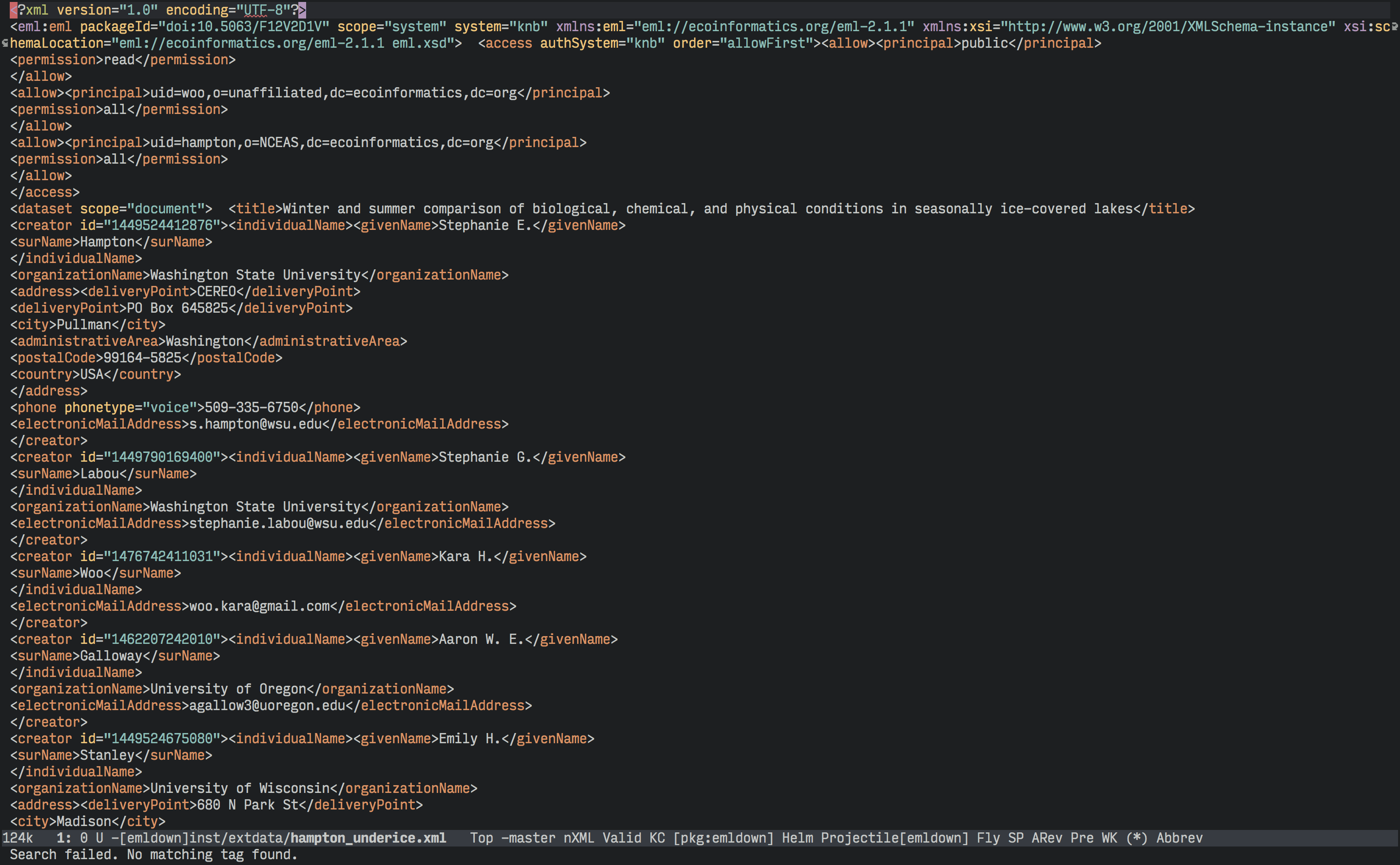
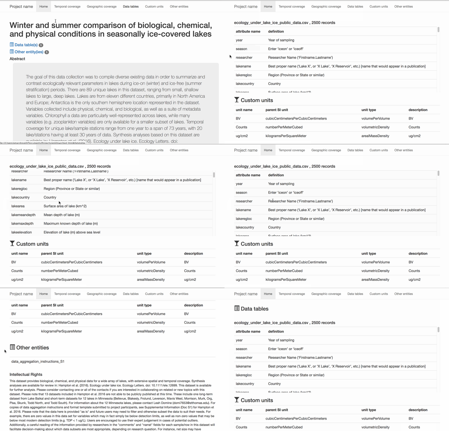
and you get something like this!

emldown

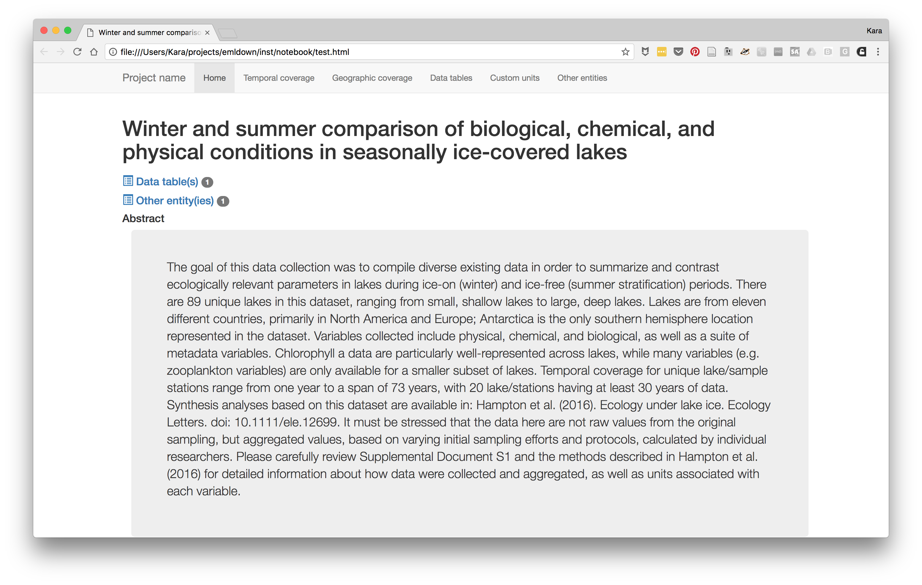
This format is much more likely to make you and your collaborators happy because it's more engaging and easier to explore to find useful information. Note how little effort you needed to invest into making it! Viewing your metadata in this way makes it easy to read, and easy to spot any errors.

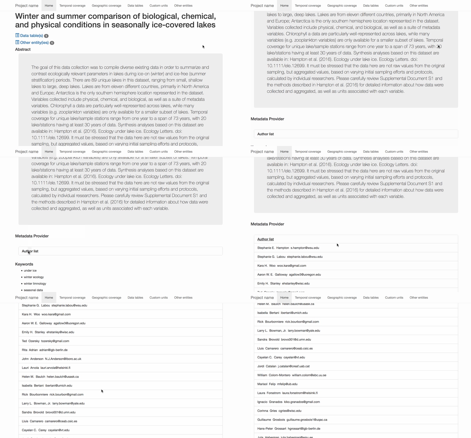
The resulting website is based on Bootstrap and has some interactive components:

demo1

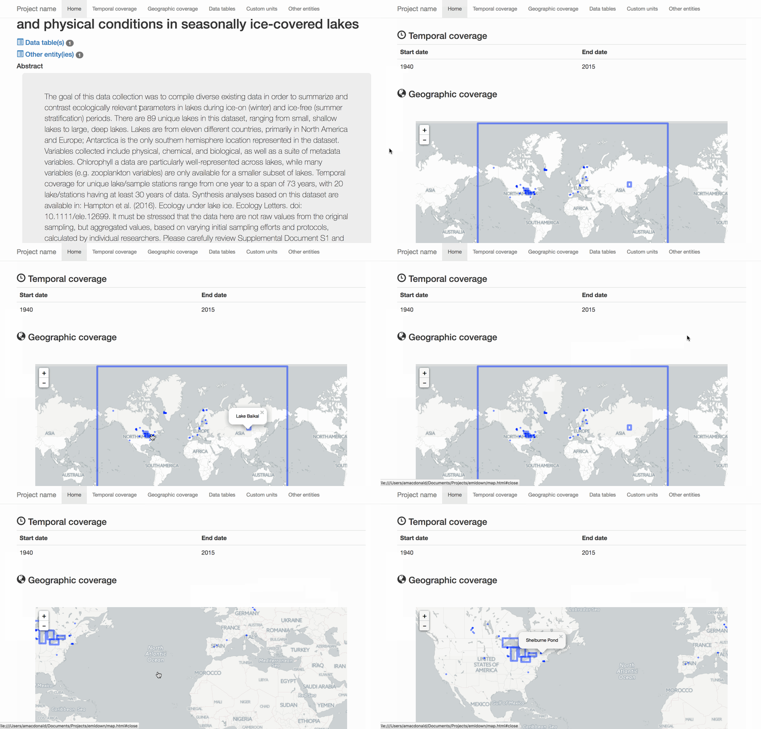
Geographic information turns into a map, made using leaflet:

demo2

Right now, we are able to capture some of the most common parts of Ecological Metadata Language, including the Title, Abstract, Authors, Keywords, Coverage (where in space and time the samples were taken), the Data Tables and Units associated with these. Over time we plan to add support for additional components of the EML specification.

demo3

You can see a live example of a website created with emldownhere

How can you contribute?

Use the package to transform the EML you have lying around on your PC into a pretty website, and if you find a bug while doing so we'll be happy to tackle it! Report any issue or feature request here, or feel free to contribute with code.

We're very happy to have been able to create this working package in two days (and thankful for that opportunity, thanks rOpenSci!); and we not-so-secretly hope that it will contribute to making writing good metadata more attractive and therefore more common.

elastic - Elasticsearch for R

$
0
0

elastic is an R client for Elasticsearch

elastic has been around since 2013, with the first commit in November, 2013.

sidebar - 'elastic' was picked as a package named before the company now known as Elastic changed their name to Elastic.

What is Elasticsearch?

If you aren't familiar with Elasticsearch, it is a distributed, RESTful search and analytics engine. It's similar to Solr. It falls in the NoSQL bin of databases, holding data in JSON documents, instead of rows and columns. Elasticsearch has a concept of index, similar to a database in SQL-land. You can hold many documents of similar type within a single index. There is powerful search capabilities, including lots of different types of queries that can be done separately or combined. And best of all it's super fast.

Other clients

The Elastic company maintains some official clients, including the Python clientelasticsearch-py, and it's higher level DSL client elasticsearch-dsl.

I won't talk much about it, but we have slowly been working on an R equivalent of the Python DSL client, called elasticdsl, for a human friendly way to compose Elasticsearch queries.

Vignettes

Check out the elastic introduction vignette and the search vignette to get started.

Noteable features

  • elastic has nearly complete coverage of the Elasticsearch HTTP API. If there's anything missing you need in this client, let us know! Check out thefeatures label for features we plan to add to the package.
  • We fail well. This is important to us. We allow the user to choose simple errors to just give e.g., 404 HTTP error, or complex errors, including full stack trace from Elasticsearch in addition to the HTTP errror. We strive to fail well when users give the wrong type of input, etc. as well. Let us know if elastic is not failing well!
  • We strive to allow R centric ways of interacting with Elasticsearch. For example, in the function docs_bulk, our interface to the Elasticsearch bulk API we make it easy to create documents in your Elasticsearch instance from R lists, data.frame's and from bulk format files on disk.
  • elastic works with most versions of Elasticsearch. We run the test suite on 11 versions of Elasticsearch, from v1.0.0 up to v5.5.0. We strive to fail well with useful messages when there is a feature no longer available or one that is a new feature and not available in previous Elasticsearch versions.
  • Search inputs are flexible: lists and JSON strings both work.
  • Arguably, a noteable feature is that this client has been around nearly 4 years, so we've surfaced and squashed many bugs.

Getting help


Setup

Install elastic

install.packages("elastic")

Or get the development version:

devtools::install_github("ropensci/elastic")
library(elastic)

I'm running Elasticsearch version:

ping()$version$number#> [1] "5.4.0"

Examples

Initialize a client

Using connect()

elastic::connect()#> transport:  http#> host:       127.0.0.1#> port:       9200#> path:       NULL#> username:   NULL#> password:   <secret>#> errors:     simple#> headers (names):  NULL

By default, you connect to localhost and port 9200. There's paramaters for setting transport schema, username, password, and base search path (e.g.,_search or something else).

See bottom of post about possible changes in connections.

Get some data

Elasticsearch has a bulk load API to load data in fast. The format is pretty weird though. It's sort of JSON, but would pass no JSON linter. I include a few data sets in elastic so it's easy to get up and running, and so when you run examples in this package they'll actually run the same way (hopefully).

Public Library of Science (PLOS) data

A dataset inluded in the elastic package is metadata for PLOS scholarly articles. Get the file path, then load:

plosdat <-system.file("examples","plos_data.json", package ="elastic")invisible(docs_bulk(plosdat))

The main search function is Search(). Running it without any inputs searches across all indices - in this case only the plos index.

Search()
#> $took
#> [1] 1
#>
#> $timed_out
#> [1] FALSE
#>
#> $`_shards`
#> $`_shards`$total
#> [1] 5
#>
#> $`_shards`$successful
#> [1] 5
#>
#> $`_shards`$failed
#> [1] 0
...

Search just the plos index and only return 1 result

Search(index ="plos", size =1)$hits$hits#> [[1]]#> [[1]]$`_index`#> [1] "plos"#>#> [[1]]$`_type`#> [1] "article"#>#> [[1]]$`_id`#> [1] "0"#>#> [[1]]$`_score`#> [1] 1#>#> [[1]]$`_source`#> [[1]]$`_source`$id#> [1] "10.1371/journal.pone.0007737"#>#> [[1]]$`_source`$title#> [1] "Phospholipase C-β4 Is Essential for the Progression of the Normal Sleep Sequence and Ultradian Body Temperature Rhythms in Mice"

Search the plos index, and the article document type, sort by title, and query for antibody, limit to 1 result.

First, with Elasticsearch v5 and greater, we need to set fielddata = true if we want to search on or sort on a text field.

mapping_create("plos","article", update_all_types =TRUE, body ='{"properties": {"title": {"type":     "text","fielddata": true   } }}')#> $acknowledged#> [1] TRUE
Search(index ="plos", type ="article", sort ="title", q ="antibody", size =1)$hits$hits#> [[1]]#> [[1]]$`_index`#> [1] "plos"#>#> [[1]]$`_type`#> [1] "article"#>#> [[1]]$`_id`#> [1] "568"#>#> [[1]]$`_score`#> NULL#>#> [[1]]$`_source`#> [[1]]$`_source`$id#> [1] "10.1371/journal.pone.0085002"#>#> [[1]]$`_source`$title#> [1] "Evaluation of 131I-Anti-Angiotensin II Type 1 Receptor Monoclonal Antibody as a Reporter for Hepatocellular Carcinoma"#>#>#> [[1]]$sort#> [[1]]$sort[[1]]#> [1] "1"

Get documents

Get document with id=1

docs_get(index ='plos', type ='article', id =1)#> $`_index`#> [1] "plos"#>#> $`_type`#> [1] "article"#>#> $`_id`#> [1] "1"#>#> $`_version`#> [1] 1#>#> $found#> [1] TRUE#>#> $`_source`#> $`_source`$id#> [1] "10.1371/journal.pone.0098602"#>#> $`_source`$title#> [1] "Population Genetic Structure of a Sandstone Specialist and a Generalist Heath Species at Two Levels of Sandstone Patchiness across the Strait of Gibraltar"

Get certain fields

docs_get(index ='plos', type ='article', id =1, fields ='id')#> $`_index`#> [1] "plos"#>#> $`_type`#> [1] "article"#>#> $`_id`#> [1] "1"#>#> $`_version`#> [1] 1#>#> $found#> [1] TRUE

Raw JSON data

You can optionally get back raw JSON from many functions by setting parameter raw=TRUE.

For example, get raw JSON, then parse with jsonlite

(out <- docs_mget(index ="plos", type ="article", id =5:6, raw =TRUE))#> [1] "{\"docs\":[{\"_index\":\"plos\",\"_type\":\"article\",\"_id\":\"5\",\"_version\":1,\"found\":true,\"_source\":{\"id\":\"10.1371/journal.pone.0085123\",\"title\":\"MiR-21 Is under Control of STAT5 but Is Dispensable for Mammary Development and Lactation\"}},{\"_index\":\"plos\",\"_type\":\"article\",\"_id\":\"6\",\"_version\":1,\"found\":true,\"_source\":{\"id\":\"10.1371/journal.pone.0098600\",\"title\":\"Correction: Designing Mixed Species Tree Plantations for the Tropics: Balancing Ecological Attributes of Species with Landholder Preferences in the Philippines\"}}]}"#> attr(,"class")#> [1] "elastic_mget"
jsonlite::fromJSON(out)#> $docs#>   _index   _type _id _version found                   _source.id#> 1   plos article   5        1  TRUE 10.1371/journal.pone.0085123#> 2   plos article   6        1  TRUE 10.1371/journal.pone.0098600#>                                                                                                                                                     _source.title#> 1                                                                       MiR-21 Is under Control of STAT5 but Is Dispensable for Mammary Development and Lactation#> 2 Correction: Designing Mixed Species Tree Plantations for the Tropics: Balancing Ecological Attributes of Species with Landholder Preferences in the Philippines

Here, we'll use another dataset that comes with the package on Shakespeare plays.

gbifdat <-system.file("examples","gbif_data.json", package ="elastic")invisible(docs_bulk(gbifdat))

Define an aggregation query:

aggs <-'{"aggs": {"latbuckets" : {"histogram" : {"field" : "decimalLatitude","interval" : 5           }        }    }}'

Search the gbif index

res <- Search(index ="gbif", body = aggs, size =0)$aggregations$latbuckets$bucketsdo.call("rbind.data.frame", res)#>    key doc_count#> 2  -35         1#> 22 -30         0#> 3  -25         0#> 4  -20         0#> 5  -15         0#> 6  -10         0#> 7   -5         1#> 8    0         0#> 9    5         0#> 10  10         0#> 11  15         0#> 12  20         0#> 13  25         4#> 14  30         2#> 15  35         3#> 16  40         2#> 17  45        66#> 18  50       183#> 19  55       487#> 20  60       130#> 21  65        20

Scrolling search - instead of paging

When you want all the documents, your best bet is likely to be scrolling search.

Here's an example. First, use Search(), setting a value for the scroll parameter.

res1 <- Search(index ='shakespeare', scroll ="1m")

You get a scroll ID back when setting the scroll parameter

res1$`_scroll_id`#> [1] "DnF1ZXJ5VGhlbkZldGNoBQAAAAAAAAElFnZ2X3FJVWEyUU1HQjl2cFpWUFl0cXcAAAAAAAABJBZ2dl9xSVVhMlFNR0I5dnBaVlBZdHF3AAAAAAAAAScWdnZfcUlVYTJRTUdCOXZwWlZQWXRxdwAAAAAAAAEmFnZ2X3FJVWEyUU1HQjl2cFpWUFl0cXcAAAAAAAABIxZ2dl9xSVVhMlFNR0I5dnBaVlBZdHF3"

Use a while loop to get all results

out1 <-list()
hits <-1while(hits !=0){
  tmp1 <- scroll(scroll_id = res1$`_scroll_id`)
  hits <-length(tmp1$hits$hits)if(hits >0){
   out1 <-c(out1, tmp1$hits$hits)}}

Woohoo! Collected all 1 documents in very little time.

Now, get _source from each document:

docs <-lapply(out1,"[[","_source")length(docs)#> [1] 4988vapply(docs[1:10],"[[","","text_entry")#>  [1] "Without much shame retold or spoken of."#>  [2] "For more uneven and unwelcome news"#>  [3] "And shape of likelihood, the news was told;"#>  [4] "Mordake the Earl of Fife, and eldest son"#>  [5] "It is a conquest for a prince to boast of."#>  [6] "Amongst a grove, the very straightest plant;"#>  [7] "That some night-tripping fairy had exchanged"#>  [8] "Then would I have his Harry, and he mine."#>  [9] "This is his uncles teaching; this is Worcester,"#> [10] "Malevolent to you in all aspects;"

Bulk documents

You've already seen the bulk docs API in action above. Above though, we were using docs_bulk.character - where the input is a character string that's a file path.

Here, I'll describe briefly how you can insert any data.frame as documents in your Elasticsearch instance. We'll use the diamonds dataset from the ~54K row ggplot2 package.

#> $acknowledged
#> [1] TRUE
library(ggplot2)invisible(docs_bulk(diamonds,"diam"))#> |==================================| 100%
Search("diam")$hits$total#> [1] 47375

That's pretty easy! This function is used a lot, particularly with data.frame's - so we get many questions/feedback on this so it will just keep getting better/faster.


TO DO

Connections

We're planning to roll out changes in how you connect to Elasticsearch from elastic. Right now, you can only connect to one Elasticsearch instance per R session - your details are set and then recalled internally in each function. We plan to change this to instantiate a client and then you either call functions on the client (e.g., using R6) or pass the client object onto functions.

Checkout issue #87 to follow progress or discuss.

Move to using crul for http

crul is a relatively new R http client - and has async baked in - as well as mocking. Development should be easier with it as I can mock requests for test suites, and allow users to toggle async more easily.


Call to action

We can use your help! Elasticsearch development moves pretty fast - we'd love this client to work with every single Elasticsearch version to the extent possible - and we'd love to squash every bug and solve every feature request fast.

If you need to use Elasticsearch from R, please try out elastic!

  • Report bugs!
  • File feature requests!
  • Send PR's!

Unconf 2017: The Roads Not Taken

$
0
0

Since June, we have been highlighting the many projects that emerged from this year's rOpenSci Unconf. These projects start many weeks before unconf participants gather in-person. Each year, we ask participants to propose and discuss project ideas ahead of time in a GitHub repo. This serves to get creative juices flowing as well as help people get to know each other a bit through discussion.

This year wasn't just our biggest unconf ever, it was the biggest in terms of proposed ideas! We had more proposals than participants, so we had a great pool to draw from when we got down to work in L.A. Yet many good ideas were left on the cutting room floor. Here we highlight some of those ideas we didn't quite get to. Many have lots of potential and we hope the R and rOpenSci communities take them up!

API Interfaces

  • Many of our data access packages interface with web APIs, and our community has some ideas on how to make these easier and improve testing of these types of packages.
  • Both Amazon Web Services and Google Cloud APIs already have API wrappers, but in other languages (e.g., Java, Go), that could be wrapped to make R packages.

Development tools

Data Access

Reproducibility

Training

Publishing

  • How should R users handle reviewing and commenting R-Markdown documents.
  • What's the right blend of vignettes, R markdown templates, and parameterized reports for getting new learners up and running?
  • One of the things we hope to do more of is enable scientists to publish and get credit for their software and data. How about automating software citation, or packages for auto-submission to software or data journals?


It's Your Turn

Interested in pursuing one of these ideas? Pick up on the discussion in the project's GitHub repo and the friendly people there will welcome your contributions!

Chat with the rOpenSci team at upcoming meetings

$
0
0

You can find members of the rOpenSci team at various meetings and workshops around the world. Come say 'hi', learn about how our packages can enable your research, or about our onboarding process for contributing new packages, discuss software sustainability or tell us how we can help you do open and reproducible research.

Where's rOpenSci?

WhenWhoWhereWhat
Aug 7, 2017Scott Chamberlain, Carl Boettiger, Noam RossPortland, OREcological Society of America Annual Meeting
Aug 8, 2017Karthik RamBaltimore, MDSpace Telescope Science Institute Engineering Colloquium
Sep 12-14, 2017Jenny BryanLondon, UKEARL Conference; R-Ladies London
Sep 19-20, 2017Jenny BryanSan Francisco, CAExtending the tidyverse
Oct 1-4, 2017Scott ChamberlainOttawa, CATDWG Annual Conference
Oct 10-11, 2017Karthik Ram, Stefanie ButlandAustin, TXNumFOCUS Summit
Oct 19-21, 2017Jenny BryanLa Jolla, CAWomen in Statistics and Data Science Conference
Oct 26-27, 2017TBDMelbourne, AU2nd Annual rOpenSci AU-Unconf
Nov 7-10, 2017Scott ChamberlainDurham, NCPhenoscape Hackathon
Dec 8-9, 2017Stefanie ButlandWashington, DCAAAS Community Engagement Fellows meeting
Dec 10-14, 2017Jenny BryanAuckland, NZIASC-ARS/NZSA Conference
Dec 11, 2017Nick GoldingGhent, BEWorkshop: Developing R Packages for Accessing, Synthesizing and Analysing Ecological Data

Magick 1.0: 🎩 ✨🐇 Advanced Graphics and Image Processing in R

$
0
0

Last week, version 1.0 of the magick package appeared on CRAN: an ambitious effort to modernize and simplify high quality image processing in R. This R package builds upon the Magick++ STL which exposes a powerful C++ API to the famous ImageMagick library.

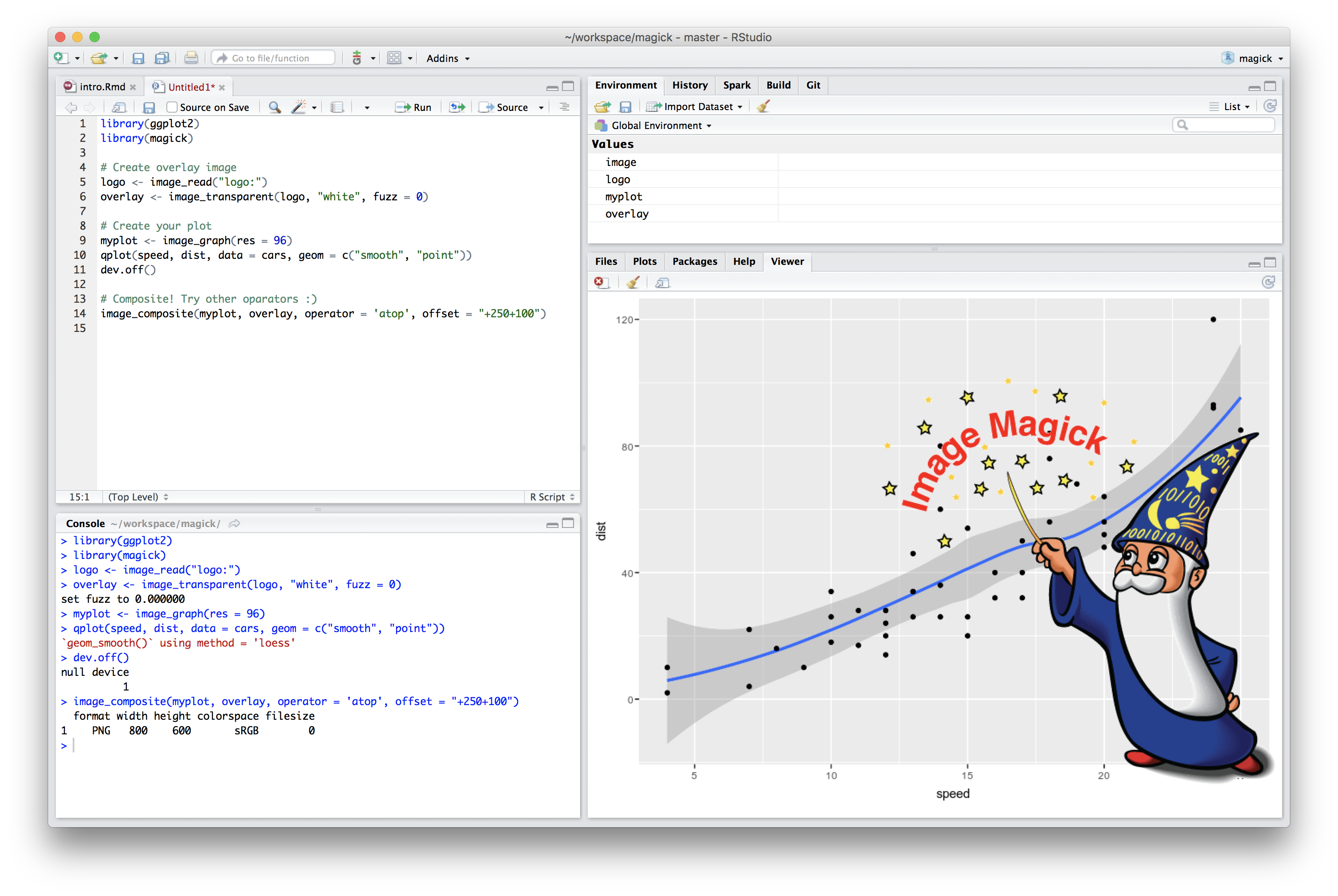
RStudio Screenshot

The best place to start learning about magick is the vignette which gives a brief overview of the overwhelming amount of functionality in this package.

Towards Release 1.0

Last year around this time rOpenSci announced the first release of the magick package: a new powerful toolkit for image reading, writing, converting, editing, transformation, annotation, and animation in R. Since the initial release there have been several updates with additional functionality, and many useRs have started to discover the power of this package to take visualization in R to the next level.

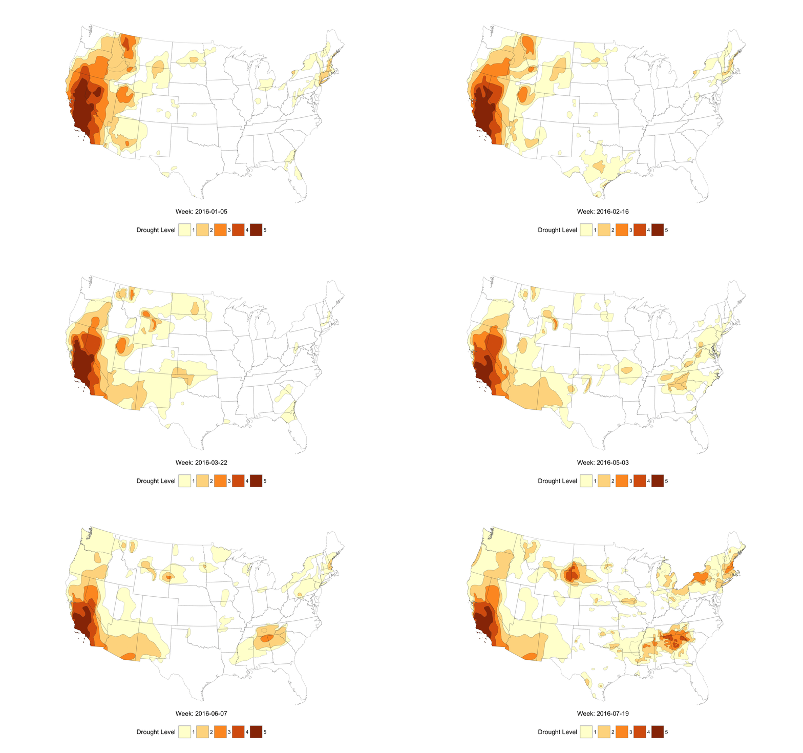
For example Bob Rudis uses magick to visualize California drought data from the U.S. Drought Monitor (click on the image to go find out more):

drought

R-ladies Lucy D'Agostino McGowan and Maëlle Salmon demonstrate how to make a beautiful collage:

collage

And Daniel P. Hadley lets Vincent Vega explains Cars:

travolta

Now, 1 year later, the 1.0 release marks an important milestone: the addition of a new native graphics device (which serves as a hybrid between a magick image object and an R plot) bridges the gap between graphics and image processing in R.

This blog post explains how the magick device allows you to seamlessly combine graphing with image processing in R. You can either use it to post-process your R graphics, or draw on imported images using the native R plotting machinery. We hope that this unified interface will make it easier to produce beautiful, reproducible images with R.

Native Magick Graphics

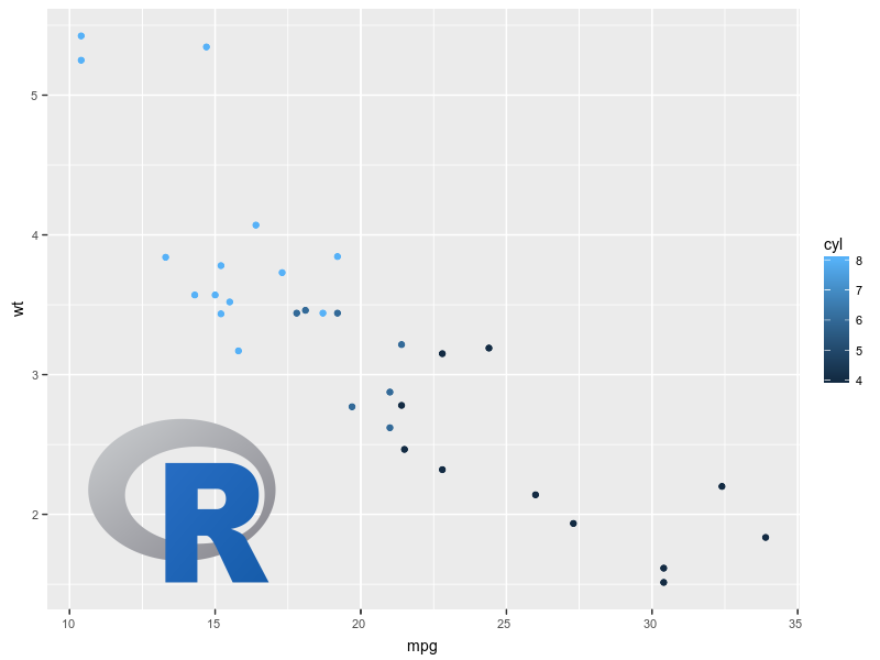
The image_graph() function opens a new graphics device similar to e.g. png() or x11(). It returns an image object to which the plot(s) will be written. Each page in the plotting device will become a frame (layer) in the image object.

# Produce image using graphics device
fig <- image_graph(res =96)
ggplot2::qplot(mpg, wt, data = mtcars, colour = cyl)
dev.off()

The fig object now contains the image that we can easily post-process. For example we can overlay another image:

logo <- image_read("https://www.r-project.org/logo/Rlogo.png")
out <- image_composite(fig, image_scale(logo,"x150"), offset ="+80+380")# Show preview
image_browse(out)# Write to file
image_write(out,"myplot.png")

out

Drawing Device

The image_draw() function opens a graphics device to draw on top of an existing image using pixel coordinates.

# Open a filelibrary(magick)
frink <- image_read("https://jeroen.github.io/images/frink.png")
drawing <- image_draw(frink)

frink

We can now use R's native low-level graphics functions for drawing on top of the image:

rect(20,20,200,100, border ="red", lty ="dashed", lwd =5)
abline(h =300, col ='blue', lwd ='10', lty ="dotted")
text(10,250,"Hoiven-Glaven", family ="courier", cex =4, srt =90)
palette(rainbow(11, end =0.9))
symbols(rep(200,11),seq(0,400,40), circles = runif(11,5,35),
  bg =1:11, inches =FALSE, add =TRUE)

At any point you can inspect the current result:

image_browse(drawing)

drawing

Once you are done you can close the device and save the result.

dev.off()
image_write(drawing,'drawing.png')

By default image_draw() sets all margins to 0 and uses graphics coordinates to match image size in pixels (width x height) where (0,0) is the top left corner. Note that this means the y axis increases from top to bottom which is the opposite of typical graphics coordinates. You can override all this by passing custom xlim, ylim or mar values to image_draw().

Animated Graphics

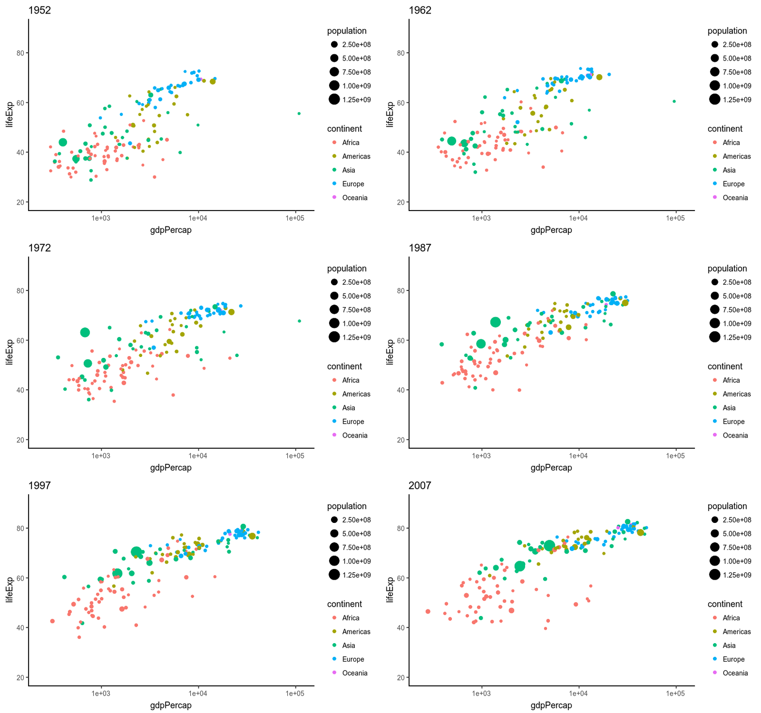
The graphics device supports multiple frames which makes it easy to create animated graphics. The example below shows how you would implement the example from the very cool gganimate package using the magick.

library(gapminder)library(ggplot2)library(magick)
img <- image_graph(res =96)
datalist <-split(gapminder, gapminder$year)
out <-lapply(datalist,function(data){
  p <- ggplot(data, aes(gdpPercap, lifeExp, size = pop, color = continent))+
    scale_size("population", limits =range(gapminder$pop))+
    scale_x_log10(limits =range(gapminder$gdpPercap))+
    geom_point()+ ylim(20,90)+  ggtitle(data$year)+ theme_classic()print(p)})
dev.off()
animation <- image_animate(img, fps =2)
image_write(animation,"animation.gif")

animation

We hope that the magick package can provide a more robust back-end for packages like gganimate to produce interactive graphics in R without requiring the user to manually install external image editing software.

Porting ImageMagick Commands to R

The magick 1.0 release now has the core image processing functionality that you expect from an image processing package. But there is still a lot of room for improvement to make magick the image processing package in R.

A lot of R users and packages currently shell out to ImageMagick command line tools for performing image manipulations. The goal is to support all these operations in the magick package, so that the images can be produced (and reproduced!) on any platform without requiring the user to install additional software.

Note that ImageMagick library is over 26 years old and has accumulated an enormous number of features in those years. Porting all of this to R is quite a bit of work, for which feedback from users is important. If there is an imagemagick operation that you like to do in R but you can't figure out how, please open an issue on GitHub. If the functionality is currently not supported yet, we will try to add it to the next version.

Image Analysis

Currently magick is focused on generating and editing images. There is yet another entirely different set of features which we like to support related to analyzing images. Image analysis can involve anything from calculating color distributions to more sophisticated feature extraction and vision tools. I am not very familiar with this field, so again we could use suggestions from users and experts.

One feature that is already available is the image_ocr() function which extracts text from the image using the rOpenSci tesseract package. Another cool example of using image analysis is the collage package which calculates color histograms to select appropriate tile images for creating a collage.

histogram

As part of supporting supporting analysis tools we plan to extract the bitmap (raster) classes into a separate package. This will enable package authors to write R extensions to analyze and manipulate on the raw image data, without necessarily depending on magick. Yet the user can always rely on magick as a powerful toolkit to import/export images and graphics into such low level bitmaps.


Tesseract and Magick: High Quality OCR in R

$
0
0

Last week we released an update of the tesseract package to CRAN. This package provides R bindings to Google's OCR library Tesseract.

install.packages("tesseract")

The new version ships with the latest libtesseract 3.05.01 on Windows and MacOS. Furthermore it includes enhancements for managing language data and using tesseract together with the magick package.

Installing Language Data

The new version has several improvements for installing additional language data. On Windows and MacOS you use the tesseract_download() function to install additional languages:

tesseract_download("fra")

Language data are now stored in rappdirs::user_data_dir('tesseract') which makes it persist across updates of the package. To OCR french text:

french <- tesseract("fra")
text <- ocr("https://jeroen.github.io/images/french_text.png", engine = french)cat(text)

Très Bien! Note that on Linux you should not use tesseract_download but instead install languages using apt-get (e.g. tesseract-ocr-fra) or yum (e.g. tesseract-langpack-fra).

Tesseract and Magick

The tesseract developers recommend to clean up the image before OCR'ing it to improve the quality of the output. This involves things like cropping out the text area, rescaling, increasing contrast, etc.

The rOpenSci magick package is perfectly suitable for this task. The latest version contains a convenient wrapper image_ocr() that works with pipes.

devtools::install_github("ropensci/magick")

Let's give it a try on some example scans:

example

# Requires devel version of magick# devtools::install_github("ropensci/magick")# Test itlibrary(magick)library(magrittr)

text <- image_read("https://courses.cs.vt.edu/csonline/AI/Lessons/VisualProcessing/OCRscans_files/bowers.jpg")%>%
  image_resize("2000")%>%
  image_convert(colorspace ='gray')%>%
  image_trim()%>%
  image_ocr()cat(text)
The Llfe and Work of
Fredson Bowers
by
G. THOMAS TANSELLE

N EVERY FIELD OF ENDEAVOR THERE ARE A FEW FIGURES WHOSE ACCOM-
plishment and influence cause them to be the symbols of their age;
their careers and oeuvres become the touchstones by which the
field is measured and its history told. In the related pursuits of
analytical and descriptive bibliography, textual criticism, and scholarly
editing, Fredson Bowers was such a figure, dominating the four decades
after 1949, when his Principles of Bibliographical Description was pub-
lished. By 1973 the period was already being called “the age of Bowers”:
in that year Norman Sanders, writing the chapter on textual scholarship
for Stanley Wells's Shakespeare: Select Bibliographies, gave this title to
a section of his essay. For most people, it would be achievement enough
to rise to such a position in a field as complex as Shakespearean textual
studies; but Bowers played an equally important role in other areas.
Editors of ninetcemh-cemury American authors, for example, would
also have to call the recent past “the age of Bowers," as would the writers
of descriptive bibliographies of authors and presses. His ubiquity in
the broad field of bibliographical and textual study, his seemingly com-
plete possession of it, distinguished him from his illustrious predeces-
sors and made him the personification of bibliographical scholarship in

his time.

\Vhen in 1969 Bowers was awarded the Gold Medal of the Biblio-
graphical Society in London, John Carter’s citation referred to the
Principles as “majestic," called Bowers's current projects “formidable,"
said that he had “imposed critical discipline" on the texts of several
authors, described Studies in Bibliography as a “great and continuing
achievement," and included among his characteristics "uncompromising
seriousness of purpose” and “professional intensity." Bowers was not
unaccustomed to such encomia, but he had also experienced his share of
attacks: his scholarly positions were not universally popular, and he
expressed them with an aggressiveness that almost seemed calculated to

Not bad but not perfect. Can you do a better job?

So you (don't) think you can review a package

$
0
0

Contributing to an open-source community without contributing code is an oft-vaunted idea that can seem nebulous. Luckily, putting vague ideas into action is one of the strengths of the rOpenSci Community, and their package onboarding system offers a chance to do just that.

This was my first time reviewing a package, and, as with so many things in life, I went into it worried that I'd somehow ruin the package-reviewing process— not just the package itself, but the actual onboarding infrastructure...maybe even rOpenSci on the whole.

Barring the destruction of someone else's hard work and/or an entire organization, I was fairly confident that I'd have little to offer in the way of useful advice. What if I have absolutely nothing to say other than, yes, this is, in fact, a package?!

rOpenSci package review: what I imagined

So, step one (for me) was: confess my inadequacies and seek advice. It turns out that much of the advice vis-à-vis how to review a package is baked right into the documents. The reviewer template is a great trail map, the utility of which is fleshed out in the rOpenSci Package Reviewing Guide. Giving these a thorough read, and perusing a recommended review or two (links in the reviewing guide) will probably have you raring to go. But, if you're feeling particularly neurotic (as I almost always am), the rOpenSci onboarding editors and larger community are endless founts of wisdom and resources.

visdat📦👀

I knew nothing about Nicholas Tierney's visdat package prior to receiving my invitation to review it. So the first (coding-y) thing I did was play around with it in the same way I do for other cool R packages I encounter. This is a totally unstructured mish-mash of running examples, putting my own data in, and seeing what happens. In addition to being amusing, it's a good way to sort of "ground-truth" the package's mission, and make sure there isn't some super helpful feature that's going unsung.

If you're not familiar with visdat, it "provides a quick way for the user to visually examine the structure of their data set, and, more specifically, where and what kinds of data are missing."1 With early-stage EDA (exploratory data analysis), you're really trying to get a feel of your data. So, knowing that I couldn't be much help in the "here's how you could make this faster with C++" department, I decided to fully embrace my role as "naïve user".2

Questions I kept in mind as ~myself~ resident naïf:

  • What did I think this thing would do? Did it do it?
  • What are things that scare me off?

The latter question is key, and, while I don't have data to back this up, can be a sort of "silent" usability failure when left unexamined. Someone who tinkers with a package, but finds it confusing doesn't necessarily stop to give feedback. There's also a pseudo curse-of-knowledge component. While messages and warnings are easily parsed, suppressed, dealt with, and/or dismissed by the veteran R user/programmer, unexpected, brightly-coloured text can easily scream Oh my gosh you broke it all!! to those with less experience.

Myriad lessons learned 💡

I can't speak for Nick per the utility or lack thereof of my review (you can see his take here, but I can vouch for the package-reviewing experience as a means of methodically inspecting the innards of an R package. Methodical is really the operative word here. Though "read the docs," or "look at the code" sounds straight-forward enough, it's not always easy to coax oneself into going through the task piece-by-piece without an end goal in mind. While a desire to contribute to open-source software is noble enough (and is how I personaly ended up involved in this process-- with some help/coaxing from Noam Ross), it's also an abstraction that can leave one feeling overwhelmed, and not knowing where to begin.3

There are also self-serving bonus points that one simply can't avoid, should you go the rOpenSci-package-reviewing route-- especially if package development is new to you.4 Heck, the package reviewing guide alone was illuminating.

Furthermore, the wise-sage 🦉 rOpenSci onboarding editors5 are excellent matchmakers, and ensure that you're actually reviewing a package authored by someone who wants their package to be reviewed. This sounds simple enough, but it's a comforting thought to know that your feedback isn't totally unsolicited.


  1. Yes, I'm quoting my own review. 

  2. So, basically just playing myself... Also I knew that, if nothing more, I can proofread and copy edit. 

  3. There are lots of good resources out there re. overcoming this obstacle, though (e.g. First Timers Only; or Charlotte Wickham's Collaborative Coding from useR!2017 is esp. 👍 for the R-user). 

  4. OK, so I don't have a parallel world wherein a very experienced package-developer version of me is running around getting less out of the process, but if you already deeply understand package structure, you're unlikely to stumble upon quite so many basic "a-ha" moments. 

  5. 👋 Noam Ross, Scott Chamberlain, Karthik Ram, & Maëlle Salmon 

Onboarding visdat, a tool for preliminary visualisation of whole dataframes

$
0
0

Take a look at the data

This is a phrase that comes up when you first get a dataset.

It is also ambiguous. Does it mean to do some exploratory modelling? Or make some histograms, scatterplots, and boxplots? Is it both?

Starting down either path, you often encounter the non-trivial growing pains of working with a new dataset. The mix ups of data types - height in cm coded as a factor, categories are numerics with decimals, strings are datetimes, and somehow datetime is one long number. And let's not forget everyone's favourite: missing data.

These growing pains often get in the way of your basic modelling or graphical exploration. So, sometimes you can't even start to take a look at the data, and that is frustrating.

The visdat package aims to make this preliminary part of analysis easier. It focuses on creating visualisations of whole dataframes, to make it easy and fun for you to "get a look at the data".

Making visdat was fun, and it was easy to use. But I couldn't help but think that maybe visdat could be more.

  • I felt like the code was a little sloppy, and that it could be better.
  • I wanted to know whether others found it useful.

What I needed was someone to sit down and read over it, and tell me what they thought. And hey, a publication out of this would certainly be great.

Too much to ask, perhaps? No. Turns out, not at all. This is what the rOpenSci onboarding process provides.

rOpenSci onboarding basics

Onboarding a package onto rOpenSci is an open peer review of an R package. If successful, the package is migrated to rOpenSci, with the option of putting it through an accelerated publication with JOSS.

What's in it for the author?

  • Feedback on your package
  • Support from rOpenSci members
  • Maintain ownership of your package
  • Publicity from it being under rOpenSci
  • Contribute something to rOpenSci
  • Potentially a publication

What can rOpenSci do that CRAN cannot?

The rOpenSci onboarding process provides a stamp of quality on a package that you do not necessarily get when a package is on CRAN 1. Here's what rOpenSci does that CRAN cannot:

  • Assess documentation readability / usability
  • Provide a code review to find weak points / points of improvement
  • Determine whether a package is overlapping with another.

So I submitted visdat to the onboarding process. For me, I did this for three reasons.

  1. So visdat could become a better package
  2. Pending acceptance, I would get a publication in JOSS
  3. I get to contribute back to rOpenSci

Submitting the package was actually quite easy - you go to submit an issue on the onboarding page on GitHub, and it provides a magical template for you to fill out 2, with no submission gotchas - this could be the future 3. Within 2 days of submitting the issue, I had a response from the editor, Noam Ross, and two reviewers assigned, Mara Averick, and Sean Hughes.

I submitted visdat and waited, somewhat apprehensively. What would the reviewers think?

In fact, Mara Averick wrote a post: "So you (don't) think you can review a package" about her experience evaluating visdat as a first-time reviewer.

Getting feedback

Unexpected extras from the review

Even before the review started officially, I got some great concrete feedback from Noam Ross, the editor for the visdat submission.

  • Noam used the goodpractice package, to identify bad code patterns and other places to immediately improve upon in a concrete way. This resulted in me:
    • Fixing error prone code such as using 1:length(...), or 1:nrow(...)
    • Improving testing using the visualisation testing software vdiffr)
    • Reducing long code lines to improve readability
    • Defining global variables to avoid a NOTE ("no visible binding for global variable")

So before the review even started, visdat is in better shape, with 99% test coverage, and clearance from goodpractice.

The feedback from reviewers

I received prompt replies from the reviewers, and I got to hear really nice things like "I think visdat is a very worthwhile project and have already started using it in my own work.", and "Having now put it to use in a few of my own projects, I can confidently say that it is an incredibly useful early step in the data analysis workflow. vis_miss(), in particular, is helpful for scoping the task at hand ...". In addition to these nice things, there was also great critical feedback from Sean and Mara.

A common thread in both reviews was that the way I initially had visdat set up was to have the first row of the dataset at the bottom left, and the variable names at the bottom. However, this doesn't reflect what a dataframe typically looks like - with the names of the variables at the top, and the first row also at the top. There was also suggestions to add the percentage of missing data in each column.

On the left are the old visdat and vismiss plots, and on the right are the new visdat and vismiss plots.

Changing this makes the plots make a lot more sense, and read better.

Mara made me aware of the warning and error messages that I had let crop up in the package. This was something I had grown to accept - the plot worked, right? But Mara pointed out that from a user perspective, seeing these warnings and messages can be a negative experience for the user, and something that might stop them from using it - how do they know if their plot is accurate with all these warnings? Are they using it wrong?

Sean gave practical advice on reducing code duplication, explaining how to write general construction method to prepare the data for the plots. Sean also explained how to write C++ code to improve the speed of vis_guess().

From both reviewers I got nitty gritty feedback about my writing - places where documentation that was just a bunch of notes I made, or where I had reversed the order of a statement.

What did I think?

I think that getting feedback in general on your own work can be a bit hard to take sometimes. We get attached to our ideas, we've seen them grow from little thought bubbles all the way to "all growed up" R packages. I was apprehensive about getting feedback on visdat. But the feedback process from rOpenSci was, as Tina Turner put it, "simply the best".

Boiling down the onboarding review process down to a few key points, I would say it is transparent, friendly, and thorough.

Having the entire review process on GitHub means that everyone is accountable for what they say, and means that you can track exactly what everyone said about it in one place. No email chain hell with (mis)attached documents, accidental reply-alls or single replies. The whole internet is cc'd in on this discussion.

Being an rOpenSci initiative, the process is incredibly friendly and respectful of everyone involved. Comments are upbeat, but are also, importantly thorough, providing constructive feedback.

So what does visdat look like?

library(visdat)

vis_dat(airquality)

visdat-example

This shows us a visual analogue of our data, the variable names are shown on the top, and the class of each variable is shown, along with where missing data.

You can focus in on missing data with vis_miss()

vis_miss(airquality)

vis-miss-example

This shows only missing and present information in the data. In addition to vis_dat() it shows the percentage of missing data for each variable and also the overall amount of missing data. vis_miss() will also indicate when a dataset has no missing data at all, or a very small percentage.

The future of visdat

There are some really exciting changes coming up for visdat. The first is making a plotly version of all of the figures that provides useful tooltips and interactivity. The second and third changes to bring in later down the track are to include the idea of visualising expectations, where the user can search their data for particular things, such as particular characters like "~" or values like -99, or -0, or conditions "x > 101", and visualise them. Another final idea is to make it easy to visually compare two dataframes of differing size. We also want to work on providing consistent palettes for particular datatypes. For example, character, numerics, integers, and datetime would all have different (and consistently different) colours.

I am very interested to hear how people use visdat in their work, so if you have suggestions or feedback I would love to hear from you! The best way to leave feedback is by filing an issue, or perhaps sending me an email at nicholas [dot] tierney [at] gmail [dot] com.

The future of your R package?

If you have an R package you should give some serious thought about submitting it to the rOpenSci through their onboarding process. There are very clear guidelines on their onboarding GitHub page. If you aren't sure about package fit, you can submit a pre-submission enquiry - the editors are nice and friendly, and a positive experience awaits you!


  1. CRAN is an essential part of what makes the r-project successful and certainly without CRAN R simply would not be the language that it is today. The tasks provided by the rOpenSci onboarding require human hours, and there just isn't enough spare time and energy amongst CRAN managers. 

  2. Never used GitHub? Don't worry, creating an account is easy, and the template is all there for you. You provide very straightforward information, and it's all there at once. 

  3. With some journals, the submission process means you aren't always clear what information you need ahead of time. Gotchas include things like "what is the residential address of every co-author", or getting everyone to sign a copyright notice. 

FedData - Getting assorted geospatial data into R

$
0
0

The package FedData has gone through software review and is now part of rOpenSci. FedData includes functions to automate downloading geospatial data available from several federated data sources (mainly sources maintained by the US Federal government).

Currently, the package enables extraction from six datasets:

FedData is designed with the large-scale geographic information system (GIS) use-case in mind: cases where the use of dynamic web-services is impractical due to the scale (spatial and/or temporal) of analysis. It functions primarily as a means of downloading tiled or otherwise spatially-defined datasets; additionally, it can preprocess those datasets by extracting data within an area of interest (AoI), defined spatially. It relies heavily on the sp, raster, and rgdal packages.

Acknowledgements

FedData is a product of SKOPE (Synthesizing Knowledge of Past Environments) and the Village Ecodynamics Project.

FedData was reviewed for rOpenSci by @jooolia, with @sckott as onboarding editor, and was greatly improved as a result.

TODO

The current CRAN version of FedData, v2.4.6, will (hopefully) be the final CRAN release of FedData 2. FedData 3 will be released in the coming months, but some code built on FedData 2 will not be compatible with FedData 3.

FedData was initially developed prior to widespread use of modern web mapping services and RESTful APIs by many Federal data-holders. Future releases of FedData will limit data transfer by utilizing server-side geospatial and data queries. We will also implement dplyr verbs, tidy data structures, (magrittr) piping, functional programming using purrr, simple features for spatial data from sf, and local data storage in OGC-compliant data formats (probably GeoJSON and NetCDF). I am also aiming for 100% testing coverage.

All that being said, much of the functionality of the FedData package could be spun off into more domain-specific packages. For example, ITRDB download functions could be part of the dplR dendrochronology package; concepts/functions having to do with the GHCN data integrated into rnoaa; and Daymet concepts integrated into daymetr. I welcome any and all suggestions about how to improve the utility of FedData; please submit an issue.

Examples

Load FedData and define a study area

# FedData Testerlibrary(FedData)library(magrittr)# Extract data for the Village Ecodynamics Project "VEPIIN" study area:# http://veparchaeology.org
vepPolygon <- polygon_from_extent(raster::extent(672800,740000,4102000,4170000),
                                  proj4string ="+proj=utm +datum=NAD83 +zone=12")

Get and plot the National Elevation Dataset for the study area

# Get the NED (USA ONLY)# Returns a raster
NED <- get_ned(template = vepPolygon,
               label ="VEPIIN")# Plot with raster::plot
raster::plot(NED)

Get and plot the Daymet dataset for the study area

# Get the DAYMET (North America only)# Returns a raster
DAYMET <- get_daymet(template = vepPolygon,
               label ="VEPIIN",
               elements =c("prcp","tmax"),
               years =1980:1985)# Plot with raster::plot
raster::plot(DAYMET$tmax$X1985.10.23)

Get and plot the daily GHCN precipitation data for the study area

# Get the daily GHCN data (GLOBAL)# Returns a list: the first element is the spatial locations of stations,# and the second is a list of the stations and their daily data
GHCN.prcp <- get_ghcn_daily(template = vepPolygon,
                            label ="VEPIIN",
                            elements =c('prcp'))# Plot the NED again
raster::plot(NED)# Plot the spatial locations
sp::plot(GHCN.prcp$spatial,
         pch =1,
         add =TRUE)
legend('bottomleft',
       pch =1,
       legend="GHCN Precipitation Records")

Get and plot the daily GHCN temperature data for the study area

# Elements for which you require the same data# (i.e., minimum and maximum temperature for the same days)# can be standardized using standardize==T
GHCN.temp <- get_ghcn_daily(template = vepPolygon,
                            label ="VEPIIN",
                            elements =c('tmin','tmax'),
                            years =1980:1985,
                            standardize =TRUE)# Plot the NED again
raster::plot(NED)# Plot the spatial locations
sp::plot(GHCN.temp$spatial,
         add =TRUE,
         pch =1)
legend('bottomleft',
       pch =1,
       legend ="GHCN Temperature Records")

Get and plot the National Hydrography Dataset for the study area

# Get the NHD (USA ONLY)
NHD <- get_nhd(template = vepPolygon,
               label ="VEPIIN")# Plot the NED again
raster::plot(NED)# Plot the NHD data
NHD %>%lapply(sp::plot,
         col ='black',
         add =TRUE)

Get and plot the NRCS SSURGO data for the study area

# Get the NRCS SSURGO data (USA ONLY)
SSURGO.VEPIIN <- get_ssurgo(template = vepPolygon,
                     label ="VEPIIN")#> Warning: 1 parsing failure.#> row # A tibble: 1 x 5 col     row     col               expected actual expected   <int>   <chr>                  <chr>  <chr> actual 1  1276 slope.r no trailing characters     .5 file # ... with 1 more variables: file <chr># Plot the NED again
raster::plot(NED)# Plot the SSURGO mapunit polygons
plot(SSURGO.VEPIIN$spatial,
     lwd =0.1,
     add =TRUE)

Get and plot the NRCS SSURGO data for particular soil survey areas

# Or, download by Soil Survey Area names
SSURGO.areas <- get_ssurgo(template =c("CO670","CO075"),
                           label ="CO_TEST")# Let's just look at spatial data for CO675
SSURGO.areas.CO675 <- SSURGO.areas$spatial[SSURGO.areas$spatial$AREASYMBOL=="CO075",]# And get the NED data under them for pretty plotting
NED.CO675 <- get_ned(template = SSURGO.areas.CO675,
                            label ="SSURGO_CO675")# Plot the SSURGO mapunit polygons, but only for CO675
plot(NED.CO675)
plot(SSURGO.areas.CO675,
     lwd =0.1,
     add =TRUE)

Get and plot the ITRDB chronology locations in the study area

# Get the ITRDB records
ITRDB <- get_itrdb(template = vepPolygon,
                        label ="VEPIIN",
                        makeSpatial =TRUE)# Plot the NED again
raster::plot(NED)# Map the locations of the tree ring chronologies
plot(ITRDB$metadata,
     pch =1,
     add =TRUE)
legend('bottomleft',
       pch =1,
       legend ="ITRDB chronologies")

Onboarding visdat, a tool for preliminary visualisation of whole dataframes

$
0
0

Take a look at the data

This is a phrase that comes up when you first get a dataset.

It is also ambiguous. Does it mean to do some exploratory modelling? Or make some histograms, scatterplots, and boxplots? Is it both?

Starting down either path, you often encounter the non-trivial growing pains of working with a new dataset. The mix ups of data types - height in cm coded as a factor, categories are numerics with decimals, strings are datetimes, and somehow datetime is one long number. And let’s not forget everyone’s favourite: missing data.

These growing pains often get in the way of your basic modelling or graphical exploration. So, sometimes you can’t even start to take a look at the data, and that is frustrating.

The visdat package aims to make this preliminary part of analysis easier. It focuses on creating visualisations of whole dataframes, to make it easy and fun for you to “get a look at the data”.

Making visdat was fun, and it was easy to use. But I couldn’t help but think that maybe visdat could be more.

  • I felt like the code was a little sloppy, and that it could be better.
  • I wanted to know whether others found it useful.

What I needed was someone to sit down and read over it, and tell me what they thought. And hey, a publication out of this would certainly be great.

Too much to ask, perhaps? No. Turns out, not at all. This is what the rOpenSci onboarding process provides.

rOpenSci onboarding basics

Onboarding a package onto rOpenSci is an open peer review of an R package. If successful, the package is migrated to rOpenSci, with the option of putting it through an accelerated publication with JOSS.

What’s in it for the author?

  • Feedback on your package
  • Support from rOpenSci members
  • Maintain ownership of your package
  • Publicity from it being under rOpenSci
  • Contribute something to rOpenSci
  • Potentially a publication

What can rOpenSci do that CRAN cannot?

The rOpenSci onboarding process provides a stamp of quality on a package that you do not necessarily get when a package is on CRAN 1. Here’s what rOpenSci does that CRAN cannot:

  • Assess documentation readability / usability
  • Provide a code review to find weak points / points of improvement
  • Determine whether a package is overlapping with another.

So I submitted visdat to the onboarding process. For me, I did this for three reasons.

  1. So visdat could become a better package
  2. Pending acceptance, I would get a publication in JOSS
  3. I get to contribute back to rOpenSci

Submitting the package was actually quite easy - you go to submit an issue on the onboarding page on GitHub, and it provides a magical template for you to fill out 2, with no submission gotchas - this could be the future 3. Within 2 days of submitting the issue, I had a response from the editor, Noam Ross, and two reviewers assigned, Mara Averick, and Sean Hughes.

I submitted visdat and waited, somewhat apprehensively. What would the reviewers think?

In fact, Mara Averick wrote a post: “So you (don’t) think you can review a package” about her experience evaluating visdat as a first-time reviewer.

Getting feedback

Unexpected extras from the review

Even before the review started officially, I got some great concrete feedback from Noam Ross, the editor for the visdat submission.

  • Noam used the goodpractice package, to identify bad code patterns and other places to immediately improve upon in a concrete way. This resulted in me:
    • Fixing error prone code such as using 1:length(...), or 1:nrow(...)
    • Improving testing using the visualisation testing software vdiffr)
    • Reducing long code lines to improve readability
    • Defining global variables to avoid a NOTE (“no visible binding for global variable”)

So before the review even started, visdat is in better shape, with 99% test coverage, and clearance from goodpractice.

The feedback from reviewers

I received prompt replies from the reviewers, and I got to hear really nice things like “I think visdat is a very worthwhile project and have already started using it in my own work.“, and “Having now put it to use in a few of my own projects, I can confidently say that it is an incredibly useful early step in the data analysis workflow. vis_miss(), in particular, is helpful for scoping the task at hand …“. In addition to these nice things, there was also great critical feedback from Sean and Mara.

A common thread in both reviews was that the way I initially had visdat set up was to have the first row of the dataset at the bottom left, and the variable names at the bottom. However, this doesn’t reflect what a dataframe typically looks like - with the names of the variables at the top, and the first row also at the top. There was also suggestions to add the percentage of missing data in each column.

On the left are the old visdat and vismiss plots, and on the right are the new visdat and vismiss plots.

Changing this makes the plots make a lot more sense, and read better.

Mara made me aware of the warning and error messages that I had let crop up in the package. This was something I had grown to accept - the plot worked, right? But Mara pointed out that from a user perspective, seeing these warnings and messages can be a negative experience for the user, and something that might stop them from using it - how do they know if their plot is accurate with all these warnings? Are they using it wrong?

Sean gave practical advice on reducing code duplication, explaining how to write general construction method to prepare the data for the plots. Sean also explained how to write C++ code to improve the speed of vis_guess().

From both reviewers I got nitty gritty feedback about my writing - places where documentation that was just a bunch of notes I made, or where I had reversed the order of a statement.

What did I think?

I think that getting feedback in general on your own work can be a bit hard to take sometimes. We get attached to our ideas, we’ve seen them grow from little thought bubbles all the way to “all growed up” R packages. I was apprehensive about getting feedback on visdat. But the feedback process from rOpenSci was, as Tina Turner put it, “simply the best”.

Boiling down the onboarding review process down to a few key points, I would say it is transparent, friendly, and thorough.

Having the entire review process on GitHub means that everyone is accountable for what they say, and means that you can track exactly what everyone said about it in one place. No email chain hell with (mis)attached documents, accidental reply-alls or single replies. The whole internet is cc’d in on this discussion.

Being an rOpenSci initiative, the process is incredibly friendly and respectful of everyone involved. Comments are upbeat, but are also, importantly thorough, providing constructive feedback.

So what does visdat look like?

library(visdat)

vis_dat(airquality)

visdat-example

This shows us a visual analogue of our data, the variable names are shown on the top, and the class of each variable is shown, along with where missing data.

You can focus in on missing data with vis_miss()

vis_miss(airquality)

vis-miss-example

This shows only missing and present information in the data. In addition to vis_dat() it shows the percentage of missing data for each variable and also the overall amount of missing data. vis_miss() will also indicate when a dataset has no missing data at all, or a very small percentage.

The future of visdat

There are some really exciting changes coming up for visdat. The first is making a plotly version of all of the figures that provides useful tooltips and interactivity. The second and third changes to bring in later down the track are to include the idea of visualising expectations, where the user can search their data for particular things, such as particular characters like “~” or values like -99, or -0, or conditions “x > 101”, and visualise them. Another final idea is to make it easy to visually compare two dataframes of differing size. We also want to work on providing consistent palettes for particular datatypes. For example, character, numerics, integers, and datetime would all have different (and consistently different) colours.

I am very interested to hear how people use visdat in their work, so if you have suggestions or feedback I would love to hear from you! The best way to leave feedback is by filing an issue, or perhaps sending me an email at nicholas [dot] tierney [at] gmail [dot] com.

The future of your R package?

If you have an R package you should give some serious thought about submitting it to the rOpenSci through their onboarding process. There are very clear guidelines on their onboarding GitHub page. If you aren’t sure about package fit, you can submit a pre-submission enquiry - the editors are nice and friendly, and a positive experience awaits you!


  1. CRAN is an essential part of what makes the r-project successful and certainly without CRAN R simply would not be the language that it is today. The tasks provided by the rOpenSci onboarding require human hours, and there just isn’t enough spare time and energy amongst CRAN managers.
  2. Never used GitHub? Don’t worry, creating an account is easy, and the template is all there for you. You provide very straightforward information, and it’s all there at once.
  3. With some journals, the submission process means you aren’t always clear what information you need ahead of time. Gotchas include things like “what is the residential address of every co-author”, or getting everyone to sign a copyright notice.

FedData - Getting assorted geospatial data into R

$
0
0

The package FedData has gone through software review and is now part of rOpenSci. FedData includes functions to automate downloading geospatial data available from several federated data sources (mainly sources maintained by the US Federal government).

Currently, the package enables extraction from six datasets:

FedData is designed with the large-scale geographic information system (GIS) use-case in mind: cases where the use of dynamic web-services is impractical due to the scale (spatial and/or temporal) of analysis. It functions primarily as a means of downloading tiled or otherwise spatially-defined datasets; additionally, it can preprocess those datasets by extracting data within an area of interest (AoI), defined spatially. It relies heavily on the sp, raster, and rgdal packages.

Examples

Load FedData and define a study area

# FedData Tester
library(FedData)
library(magrittr)

# Extract data for the Village Ecodynamics Project "VEPIIN" study area:
# http://veparchaeology.org
vepPolygon <- polygon_from_extent(raster::extent(672800, 740000, 4102000, 4170000),
                                  proj4string = "+proj=utm +datum=NAD83 +zone=12")

Get and plot the National Elevation Dataset for the study area

# Get the NED (USA ONLY)
# Returns a raster
NED <- get_ned(template = vepPolygon,
               label = "VEPIIN")
# Plot with raster::plot
raster::plot(NED)

Get and plot the Daymet dataset for the study area

# Get the DAYMET (North America only)
# Returns a raster
DAYMET <- get_daymet(template = vepPolygon,
               label = "VEPIIN",
               elements = c("prcp","tmax"),
               years = 1980:1985)
# Plot with raster::plot
raster::plot(DAYMET$tmax$X1985.10.23)

Get and plot the daily GHCN precipitation data for the study area

# Get the daily GHCN data (GLOBAL)
# Returns a list: the first element is the spatial locations of stations,
# and the second is a list of the stations and their daily data
GHCN.prcp <- get_ghcn_daily(template = vepPolygon,
                            label = "VEPIIN",
                            elements = c('prcp'))
# Plot the NED again
raster::plot(NED)
# Plot the spatial locations
sp::plot(GHCN.prcp$spatial,
         pch = 1,
         add = TRUE)
legend('bottomleft',
       pch = 1,
       legend="GHCN Precipitation Records")

Get and plot the daily GHCN temperature data for the study area

# Elements for which you require the same data
# (i.e., minimum and maximum temperature for the same days)
# can be standardized using standardize==T
GHCN.temp <- get_ghcn_daily(template = vepPolygon,
                            label = "VEPIIN",
                            elements = c('tmin','tmax'),
                            years = 1980:1985,
                            standardize = TRUE)
# Plot the NED again
raster::plot(NED)
# Plot the spatial locations
sp::plot(GHCN.temp$spatial,
         add = TRUE,
         pch = 1)
legend('bottomleft',
       pch = 1,
       legend = "GHCN Temperature Records")

Get and plot the National Hydrography Dataset for the study area

# Get the NHD (USA ONLY)
NHD <- get_nhd(template = vepPolygon,
               label = "VEPIIN")
# Plot the NED again
raster::plot(NED)
# Plot the NHD data
NHD %>%
  lapply(sp::plot,
         col = 'black',
         add = TRUE)

Get and plot the NRCS SSURGO data for the study area

# Get the NRCS SSURGO data (USA ONLY)
SSURGO.VEPIIN <- get_ssurgo(template = vepPolygon,
                     label = "VEPIIN")
#> Warning: 1 parsing failure.
#> row # A tibble: 1 x 5 col     row     col               expected actual expected   <int>   <chr>                  <chr>  <chr> actual 1  1276 slope.r no trailing characters     .5 file # ... with 1 more variables: file <chr>
# Plot the NED again
raster::plot(NED)
# Plot the SSURGO mapunit polygons
plot(SSURGO.VEPIIN$spatial,
     lwd = 0.1,
     add = TRUE)

Get and plot the NRCS SSURGO data for particular soil survey areas

# Or, download by Soil Survey Area names
SSURGO.areas <- get_ssurgo(template = c("CO670","CO075"),
                           label = "CO_TEST")

# Let's just look at spatial data for CO675
SSURGO.areas.CO675 <- SSURGO.areas$spatial[SSURGO.areas$spatial$AREASYMBOL=="CO075",]

# And get the NED data under them for pretty plotting
NED.CO675 <- get_ned(template = SSURGO.areas.CO675,
                            label = "SSURGO_CO675")

# Plot the SSURGO mapunit polygons, but only for CO675
plot(NED.CO675)
plot(SSURGO.areas.CO675,
     lwd = 0.1,
     add = TRUE)

Get and plot the ITRDB chronology locations in the study area

# Get the ITRDB records
ITRDB <- get_itrdb(template = vepPolygon,
                        label = "VEPIIN",
                        makeSpatial = TRUE)
# Plot the NED again
raster::plot(NED)
# Map the locations of the tree ring chronologies
plot(ITRDB$metadata,
     pch = 1,
     add = TRUE)
legend('bottomleft',
       pch = 1,
       legend = "ITRDB chronologies")

TODO

The current CRAN version of FedData, v2.4.6, will (hopefully) be the final CRAN release of FedData 2. FedData 3 will be released in the coming months, but some code built on FedData 2 will not be compatible with FedData 3.

FedData was initially developed prior to widespread use of modern web mapping services and RESTful APIs by many Federal data-holders. Future releases of FedData will limit data transfer by utilizing server-side geospatial and data queries. We will also implement dplyr verbs, tidy data structures, (magrittr) piping, functional programming using purrr, simple features for spatial data from sf, and local data storage in OGC-compliant data formats (probably GeoJSON and NetCDF). I am also aiming for 100% testing coverage.

All that being said, much of the functionality of the FedData package could be spun off into more domain-specific packages. For example, ITRDB download functions could be part of the dplR dendrochronology package; concepts/functions having to do with the GHCN data integrated into rnoaa; and Daymet concepts integrated into daymetr. I welcome any and all suggestions about how to improve the utility of FedData; please submit an issue.

Acknowledgements

FedData is a product of SKOPE (Synthesizing Knowledge of Past Environments) and the Village Ecodynamics Project.

FedData was reviewed for rOpenSci by @jooolia, with @sckott as onboarding editor, and was greatly improved as a result.

rtimicropem: Using an *R* package as platform for harmonized cleaning of data from RTI MicroPEM air quality sensors

$
0
0

As you might remember from my blog post about ropenaq, I work as a data manager and statistician for an epidemiology project called CHAI for Cardio-vascular health effects of air pollution in Telangana, India. One of our interests in CHAI is determining exposure, and sources of exposure, to PM2.5 which are very small particles in the air that have diverse adverse health effects. You can find more details about CHAI in our recently published protocol paper. In this blog post that partly corresponds to the content of my useR! 2017 lightning talk, I’ll present a package we wrote for dealing with the output of a scientific device, which might remind you of similar issues in your experimental work.

Why write the rtimicropem package?

Part of the CHAI project is a panel study involving about 40 people wearing several devices, as you see above. The devices include a GPS, an accelerometer, a wearable camera, and a PM2.5 monitor outputting time-resolved data (the grey box on the left). Basically, with this device, the RTI MicroPEM, we get one PM2.5 exposure value every 10 seconds. This is quite exciting, right? Except that we have two main issues with it…

First of all, the output of the device, a file with a “.csv” extension corresponding to a session of measurements, in our case 24 hours of measurements, is not really a csv. The header contains information about settings of the device for that session, and then comes the actual table with measurements.

Second, since the RTI MicroPEMs are nice devices but also a work-in-progress, we had some problems with the data, such as negative relative humidity. Because of these issues, we decided to write an R package whose three goals were to:

  • Transform the output of the device into something more usable.
  • Allow the exploration of individual files after a day in the field.
  • Document our data cleaning process.

We chose R because everything else in our project, well data processing, documentation and analysis, was to be implemented in R, and because we wanted other teams to be able to use our package.

Features of rtimicropem: transform, explore and learn about data cleaning

First things first, our package lives here and is on CRAN. It has a nice documentation website thanks to pkgdown.

Transform and explore single files

In rtimicropem after the use of the convert_output function, one gets an object of the R6 class micropem class. Its fields include the settings and measurements as two data.frames, and it has methods such as summary and plot for which you see the static output below (no unit on this exploratory plot).

The plot method can also outputs an interactive graph thanks to rbokeh.

While these methods can be quite helpful to explore single files as an R user, they don’t help non R users a lot. Because we wanted members of our team working in the field to be able to explore and check files with no R knowledge, we created a Shiny app that allows to upload individual files and then look at different tabs, including one with a plot, one with the summary of measurements, etc. This way, it was easy to spot a device failure for instance, and to plan a new measurement session with the corresponding participant.

Transform a bunch of files

At the end of the CHAI data collection, we had more than 250 MicroPEM files. In order to prepare them for further processing we wrote the batch_convert function that saves the content of any number of MicroPEM files as two (real!) csv, one with the measurements, one with the settings.

Learn about data cleaning

As mentioned previously, we experienced issues with MicroPEM data quality. Although we had heard other teams complain of similar problems, in the literature there were very few details about data cleaning. We decided to gather information from other teams and the manufacturer and to document our own decisions, e.g. remove entire files based on some criteria, in a vignette of the package. This is our transparent answer to the question “What was your experience with MicroPEMs?” which we get often enough from other scientists interested in PM2.5 exposure.

Place of rtimicropem in the R package ecosystem

When preparing rtimicropem submission to rOpenSci, I started wondering whether one would like to have one R package for each scientific device out there. In our case, having the weird output to deal with, and the lack of a central data issues documentation place, were enough of a motivation. But maybe one could hope that manufacturers of scientific devices would focus a bit more on making the output format analysis-friendly, and that the open documentation of data issues would be language-agnostic and managed by the manufacturers themselves. In the meantime, we’re quite proud to have taken the time to create and share our experience with rtimicropem, and have already heard back from a few users, including one who found the package via googling “RTI MicroPEM data”! Another argument I in particular have to write R packages for dealing with scientific data is that it might motivate people to learn R, but this is maybe a bit evil.

What about the place of rtimicropem in the rOpenSci package collection? After very useful reviews by Lucy D’Agostino McGowan and Kara Woo our package got onboarded which we were really thankful for and happy about. Another package I can think off the top of my head to deal with the output of a scientific tool is plater. Let me switch roles from CHAI team member to rOpenSci onboarding co-editor here and do some advertisement… Such packages are unlikely to become the new ggplot2 but their specialization doesn’t make them less useful and they fit very well in the “data extraction” of the onboarding categories. So if you have written such a package, please consider submitting it! It’ll get better thanks to review and might get more publicity as part of a larger software ecosystem. For the rtimicropem submission we took advantage of the joint submission process of rOpenSci and the Journal of Open Source Software, JOSS, so now our piece of software has its JOSS paper with a DOI. And hopefully, having more submissions of packages for scientific hardware might inspire R users to package up the code they wrote to use the output of their scientific tools!


Community Call - rOpenSci Software Review and Onboarding

$
0
0

Are you thinking about submitting a package to rOpenSci’s open peer software review? Considering volunteering to review for the first time? Maybe you’re an experienced package author or reviewer and have ideas about how we can improve.

Join our Community Call on Wednesday, September 13th. We want to get your feedback and we’d love to answer your questions!

Agenda

  1. Welcome (Stefanie Butland, rOpenSci Community Manager, 5 min)
  2. guest: Noam Ross, editor (15 min) Noam will give an overview of the rOpenSci software review and onboarding, highlighting the role editors play and how decisions are made about policies and changes to the process.
  3. guest: Andee Kaplan, reviewer (15 min) Andee will give her perspective as a package reviewer, sharing specifics about her workflow and her motivation for doing this.
  4. Q & A (25 min, moderated by Noam Ross)

Speaker bios

Andee Kaplan is a Postdoctoral Fellow at Duke University. She is a recent PhD graduate from the Iowa State University Department of Statistics, where she learned a lot about R and reproducibility by developing a class on data stewardship for Agronomists. Andee has reviewed multiple (two!) packages for rOpenSci, iheatmapr and getlandsat, and hopes to one day be on the receiving end of the review process.

Andee on GitHub, Twitter

Noam Ross is one of rOpenSci’s four editors for software peer review. Noam is a Senior Research Scientist at EcoHealth Alliance in New York, specializing in mathematical modeling of disease outbreaks, as well as training and standards for data science and reproducibility. Noam earned his Ph.D. in Ecology from the University of California-Davis, where he founded the Davis R Users’ Group.

Noam on GitHub, Twitter

Resources

How rOpenSci uses Code Review to Promote Reproducible Science

$
0
0

At rOpenSci, we create and curate software to help scientists with the data life cycle. These tools access, download, manage, and archive scientific data in open, reproducible ways. Early on, we realized this could only be a community effort. The variety of scientific data and workflows could only be tackled by drawing on contributions of scientists with field-specific expertise.

With the community approach came challenges. How could we ensure the quality of code written by scientists without formal training in software development practices? How could we drive adoption of best practices among our contributors? How could we create a community that would support each other in this work?

We have had great success addressing these challenges via the peer review. We draw elements from a process familiar to our target community – academic peer review– and a practice from the software development world – production code review– to create a system that fosters software quality, ongoing education, and community development.

An Open Review Process

Production software review occurs within software development teams, open source or not. Contributions to a software project are reviewed by one or more other team members before incorporation into project source code. Contributions are typically small patches, and review serves as a check on quality, as well as an opportunity for training in team standards.

In academic peer review, external reviewers critique a complete product – usually a manuscript – with a very broad mandate to address any areas they see as deficient. Academic review is often anonymous and passing through it gives the product, and the author, a public mark of validation.

We blend these approaches. In our process, authors submit complete R packages to rOpenSci. Editors check that packages fit into our project’s scope, run a series of automated tests to ensure a baseline of code quality and completeness, and then assign two independent reviewers. Reviewers comment on usability, quality, and style of software code as well as documentation. Authors make changes in response, and once reviewers are satisfied with the updates, the package receives a badge of approval and joins our suite.

This process is quite iterative. After reviewers post a first round of extensive reviews, authors and reviewers chat in an informal back-and-forth, only lightly moderated by an editor. This lets both reviewers and authors pose questions of each other and explain differences of opinion. It can proceed at a much faster pace than typical academic review correspondence. We use the GitHub issues system for this conversation, and responses take minutes to days, rather than weeks to months.

The exchange is also open and public. Authors, reviewers, and editors all know each other’s identities. The broader community can view or even participate in the conversation as it happens. This provides an incentive to be thorough and provide non-adversarial, constructive reviews. Both authors and reviewers report that they enjoy and learn more from this open and direct exchange. It also has the benefit of building community. Participants have the opportunity to meaningfully network with new peers, and new collaborations have emerged via ideas spawned during the review process.

We are aware that open systems can have drawbacks. For instance, in traditional academic review, double-blind peer review can increase representation of female authors, suggesting bias in non-blind reviews. It is also possible reviewers are less critical in open review. However, we posit that the openness of the review conversation provides a check on review quality and bias; it’s harder to inject unsupported or subjective comments in public and without the cover of anonymity. Ultimately, we believe the ability of authors and reviewers to have direct but public communication improves quality and fairness.

Guidance and Standards

rOpenSci provides guidance on reviewing. This falls into two main categories: high-level best practices and low-level standards. High-level best practices are general and broadly applicable across languages and applications. These are practices such as “Write re-usable functions rather than repeating the same code,” “Test edge cases,” or “Write documentation for all of your functions.” Because of their general nature, these can be drawn from other sources and not developed from scratch. Our best practices are based on guidance originally developed by Mozilla Science Lab.

Low-level standards are specific to a language (in our case, R), applications (data interfaces) and user base (researchers). These include specific items such as naming conventions for functions, best choices of dependencies for certain tasks, and adherence to a code style guide. We have an extensive set of standards for our reviewers to check. These change over time as the R software ecosystem evolves, best practices change, and tooling and educational resources make new methods available to developers.

Our standards also change based on feedback from reviewers. We adopt into our standards suggestions that emerge in multiple reviewers across different packages. Many of these, we’ve found, have to do with with the ease-of-use and consistency of software APIs, and the type and location of information in documentation that make it easiest to find. This highlights one of the advantages of external reviewers – they can provide a fresh perspective on usability, as well as test software under different use-cases than imagined by the author.

As our standards have become more extensive, we have come to rely more on automated tools. The R ecosystem, like most languages, has a suite of tools for code linting, function testing, static code analysis and continuous integration. We require authors to use these, and editors run submissions through a suite of tests prior to sending them for review. This frees reviewers from the burden of low-level tasks to focus on high-level critiques where they can add the most value.

The Reviewer Community

One of the core challenges and rewards of our work has been developing a community of reviewers.

Reviewing is a high-skill activity. Reviewers need expertise in the programming methods used in a software package and also the scientific field of its application. (“Find me someone who knows sensory ecology and sparse data structures!”) They need good communications skills and the time and willingness to volunteer. Thankfully, the open-science and open-source worlds are filled with generous, expert people. We have been able to expand our reviewer pool as the pace of submissions and the domains of their applications have grown.

Developing the reviewer pool requires constant recruitment. Our editors actively and broadly engage with developer and research communities to find new reviewers. We recruit from authors of previous submissions, co-workers and colleagues, at conferences, through our other collaborative work and on social media. In the open-source software ecosystem, one can often identify people with particular expertise by looking at their published software or contribution to other projects, and we often will cold-email potential reviewers whose published work suggests they would be a good match for a submission.

We cultivate our reviewer pool as well as expand it. We bring back reviewers so that they may develop reviewing as a skill, but not so often as to overburden them. We provide guidance and feedback to new recruits. When assigning reviewers to a submission, we aim to pair experienced reviewers with new ones, or reviewers with expertise on a package’s programming methods with those experienced in its field of application. These reviewers learn from each other, and diversity in perspectives is an advantage; less experienced developers often provide insight that more experienced ones do not on software usability, API design, and documentation. More experienced developers will more often identify inefficiencies in code, pitfalls due to edge-cases, or suggest alternate implementation approaches.

Expanding Peer Review for Code

Code review has been one of rOpenSci’s best initiatives. We build software, build skills, and build community, and the peer review process has been a major catalyst for all three. It has made both the software we develop internally and that we accept from outside contributors more reliable, usable, and maintainable. So we are working to promote open peer review of code by more organizations working with scientific software. We helped launch The Journal of Open Source Software, which uses a version of our review process to provide a developer-friendly publication venue. JOSS’s success has led to a spin-off, the Journal of Open Source Education, which uses an open, code-review-like processes to provide feedback on curricula and educational materials. We are also developing a pilot program where software papers submitted to a partner academic journal receive a badge for going through rOpenSci review. We are encouraged by other review initiatives like ReScience and The Programming Historian. BioConductor’s code reviews, which predate ours by several years, recently switched to an open model.

If your organization is developing or curating scientific code, we believe code review, implemented well, can be a great benefit. It can take considerable effort to begin, but here are some of the key lessons we’ve learned that can help:

  • Develop standards and guidelines for your authors and reviewers to use. Borrow these freely from other projects (feel free to use ours), and modify them iteratively as you go.
  • Use automated tools such as code linters, test suites, and test coverage measures to reduce burden on authors, reviewers, and editors as much as possible.
  • Have a clear scope. Spell out to yourselves and potential contributors what your project will accept, and why. This will save a lot of confusion and effort in the future.
  • Build a community through incentives of networking, opportunities to learn, and kindness.

rOpenSci is eager to work with other groups interested in developing similar review processes, especially if you are interested in reviewing and curating scientific software in languages other than R or beyond our scope of supporting the data life cycle. Software that implements statistical algorithms, for instance, is an area ripe for open peer review of code. Please get in touch if you have questions or wish to co-pilot a review system for your project.

And of course, if you want to review, we’re always looking for volunteers. Sign up at https://ropensci.org/onboarding.


You can support rOpenSci by becoming a NumFOCUS member or making a donation to the project.

Spelling 1.0: quick and effective spell checking in R

$
0
0

The new rOpenSci spelling package provides utilities for spell checking common document formats including latex, markdown, manual pages, and DESCRIPTION files. It also includes tools especially for package authors to automate spell checking of R documentation and vignettes.

Spell Checking Packages

The main purpose of this package is to quickly find spelling errors in R packages. The spell_check_package() function extracts all text from your package manual pages and vignettes, compares it against a language (e.g. en_US or en_GB), and lists potential errors in a nice tidy format:

> spelling::spell_check_package("~/workspace/writexl")
  WORD       FOUND IN
booleans   write_xlsx.Rd:21
xlsx       write_xlsx.Rd:6,18
           title:1
           description:1

Results may contain false positives, i.e. names or technical jargon which does not appear in the English dictionary. Therefore you can create a WORDLIST file, which serves as a package-specific dictionary of allowed words:

> spelling::update_wordlist("~/workspace/writexl")
The following words will be added to the wordlist:
 - booleans
 - xlsx
Are you sure you want to update the wordlist?
1: Yes
2: No

Words added to this file are ignored in the spell check, making it easier to catch actual spelling errors:

> spell_check_package("~/workspace/writexl")
No spelling errors found.

The package also includes a cool function spell_check_setup() which adds a unit test to your package that automatically runs the spell check.

> spelling::spell_check_setup("~/workspace/writexl")
No changes required to /Users/jeroen/workspace/writexl/inst/WORDLIST
Updated /Users/jeroen/workspace/writexl/tests/spelling.R

By default this unit test will never actually fail; it merely displays potential spelling errors at the end of a R CMD check. But you can configure it to fail if you’d like, which can be useful to automatically highlight spelling errors on e.g. Travis CI.

Under the Hood

The spelling package builds on hunspell which has a fully customizable spell checking engine. Most of the code in the spelling package is dedicated to parsing and extracting text from documents before feeding it to the spell checker. For example, when spell checking an rmarkdown file, we first extract words from headers and paragraphs (but not urls or R syntax).

# Spell check this post> spelling::spell_check_files("~/workspace/roweb/_posts/2017-09-07-spelling-release.md", lang = 'en_US')
  WORD         FOUND IN
blog         2017-09-07-spelling-release.md:7
commonmark   2017-09-07-spelling-release.md:88
hunspell     2017-09-07-spelling-release.md:69
Jeroen       2017-09-07-spelling-release.md:7
knitr        2017-09-07-spelling-release.md:88
Ooms         2017-09-07-spelling-release.md:7
rmarkdown    2017-09-07-spelling-release.md:88
rOpenSci     2017-09-07-spelling-release.md:18
urls         2017-09-07-spelling-release.md:88
wordlist     2017-09-07-spelling-release.md:49
WORDLIST     2017-09-07-spelling-release.md:34

To accomplish this, we use knitr to drop code chunks, and subsequently parse markdown using commonmark and xml2, which gives us the text nodes and approximate line numbers in the source document.

The writexl package: zero dependency xlsx writer for R

$
0
0

We have started working on a new rOpenSci package called writexl. This package wraps the very powerful libxlsxwriter library which allows for exporting data to Microsoft Excel format.

The major benefit of writexl over other packages is that it is completely written in C and has absolutely zero dependencies. No Java, Perl or Rtools are required.

Getting Started

The write_xlsx function writes a data frame to an xlsx file. You can test that data roundtrips properly by reading it back using the readxl package. Columns containing dates and factors get automatically coerced to character strings.

library(writexl)
library(readxl)
write_xlsx(iris, "iris.xlsx")

# read it back
out <- read_xlsx("iris.xlsx")

You can also give it a named list of data frames, in which case each data frame becomes a sheet in the xlsx file:

write_xlsx(list(iris = iris, cars = cars, mtcars = mtcars), "mydata.xlsx")

Performance is good too; in our benchmarks writexl is about twice as fast as openxlsx:

library(microbenchmark)
library(nycflights13)
microbenchmark(
  writexl = writexl::write_xlsx(flights, tempfile()),
  openxlsx = openxlsx::write.xlsx(flights, tempfile()),
  times = 5
)
### Unit: seconds
###      expr       min        lq      mean    median        uq       max neval
###   writexl  8.884712  8.904431  9.103419  8.965643  9.041565  9.720743     5
###  openxlsx 17.166818 18.072527 19.171003 18.669805 18.756661 23.189206     5

Roadmap

The initial version of writexl implements the most important functionality for R users: exporting data frames. However the underlying libxlsxwriter library actually provides far more sophisticated functionality such as custom formatting, writing complex objects, formulas, etc.

Most of this probably won’t be useful to R users. But if you have a well defined use case for exposing some specific features from the library in writexl, open an issue on Github and we’ll look into it!

Experiences as a first time rOpenSci package reviewer

$
0
0

It all started January 26th this year when I signed up to volunteer as a reviewer for R packages submitted to rOpenSci. My main motivation for wanting to volunteer was to learn something new and to contribute to the R open source community. If you are wondering why the people behind rOpenSci are doing this, you can read How rOpenSci uses Code Review to Promote Reproducible Science.

Three months later I was contacted by Maelle Salmon asking whether I was interested in reviewing the R package patentsview for rOpenSci. And yes, I was! To be honest I was a little bit thrilled.

The packages are submitted for review to rOpenSci via an issue to their GitHub repository and also the reviews happen there. So you can check outall previous package submissions and reviews. With all the information you get from rOpenSci and also the help from the editor it is straightforward to do the package review. Before I started I read the reviewer guides (links below) and checked out a few of the existing reviews. I installed the package patentsview from GitHub and also downloaded the source code so I could check out how it was implemented.

I started by testing core functionality of the package by running the examples that were mentioned in the README of the package. I think this is a good starting point because you get a feeling of what the author wants to achieve with the package. Later on I came up with my own queries (side note: this R package interacts with an API from which you can query patents). During the process I used to switch between writing queries like a normal user of the package would do and checking the code. When I saw something in the code that wasn’t quite clear to me or looked wrong I went back to writing new queries to check whether the behavior of the methods was as expected.

With this approach I was able to give feedback to the package author which led to the inclusion of an additional unit test, a helper function that makes the package easier to use, clarification of an error message and an improved documentation. You can find the review I did here.

There are several R packages that helped me get started with my review, e.g. devtools andgoodpractice. These packages can also help you when you start writing your own packages. An example for a very useful method is devtools::spell_check(), which performs a spell check on the package description and on manual pages. At the beginning I had an issue with goodpractice::gp() but Maelle Salmon (the editor) helped me resolve it.

In the rest of this article you can read what I gained personally from doing a review.

Contributing to the open source community

When people think about contributing to the open source community, the first thought is about creating a new R package or contributing to one of the major packages out there. But not everyone has the resources (e.g. time) to do so. You also don’t have awesome ideas every other day which can immediately be implemented into new R packages to be used by the community. Besides contributing with code there are also lots of other things than can be useful for other R users, for example writing blog posts about problems you solved, speaking at meetups or reviewing code to help improve it. What I like much about reviewing code is that people see things differently and have other experiences. As a reviewer, you see a new package from the user’s perspective which can be hard for the programmer themselves. Having someone else review your code helps finding things that are missing because they seem obvious to the package author or detect code pieces that require more testing. I had a great feeling when I finished the review, since I had helped improve an already amazing R package a little bit more.

Reviewing helps improve your own coding style

When I write R code I usually try to do it in the best way possible.Google’s R Style Guide is a good start to get used to coding best practice in R and I also enjoyed reading Programming Best Practices Tidbits. So normally when I think some piece of code can be improved (with respect to speed, readability or memory usage) I check online whether I can find a better solution. Often you just don’t think something can be improved because you always did it in a certain way or the last time you checked there was no better solution. This is when it helps to follow other people’s code. I do this by reading their blogs, following many R users on Twitter and checking their GitHub account. Reviewing an R package also helped me a great deal with getting new ideas because I checked each function a lot more carefully than when I read blog posts. In my opinion, good code does not only use the best package for each problem but also the small details are well implemented. One thing I used to do wrong for a long time was filling of data.frames until I found a better (much faster)solution on stackoverflow. And with respect to this you can learn a lot from someone else’s code. What I found really cool in the package I reviewed was the usage of small helper functions (seeutils.R). Functions like paste0_stop and paste0_message make the rest of the code a lot easier to read.

Good start for writing your own packages

When reviewing an R package, you check the code like a really observant user. I noticed many things that you usually don’t care about when using an R package, like comments, how helpful the documentation and the examples are, and also how well unit tests cover the code. I think that reviewing a few good packages can prepare you very well for writing your own packages.

Do you want to contribute to rOpenSci yourself?

If I motivated you to become an rOpenSci reviewer, please sign up! Here is a list of useful things if you want to become an rOpenSci reviewer like me.

If you are generally interested in either submitting or reviewing an R package, I would like to invite you to the Community Call on rOpenSci software review and onboarding.

Viewing all 668 articles
Browse latest View live